
In this Level, we will introduce the ALLSELECTED() function. ALLSELECTED() is popular for its support of “visual totals” in our queries, and is prominent in the world of Power BI. It is member of the Filter functions group in DAX, and, like ALL() and other functions within this group, serves as a useful tool in the manipulation of context. Regardless of axes selected and filters employed within our reports, we often have a need to modify the overall context, as we’ll see again in this Level. ALLSELECTED() makes the presentation of “situational context” within a larger context sophisticated, yet straightforward.
We’ll introduce ALLSELECTED() within the setting of a common business need in this Level, and likely come across it again in various uses as we progress through the Stairway to DAX and Power BI. Our focus in this Level will be the use of ALLSELECTED() to generate “visual totals” within simple visuals.
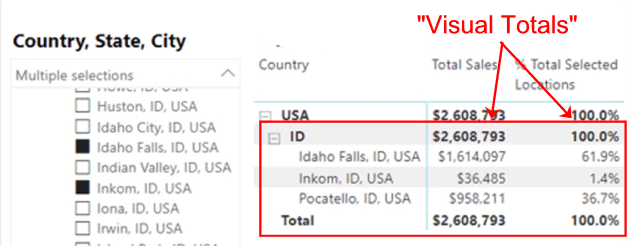
Illustration 1: Consider ALLSELECTED() for “Visual Totals…”
As a part of our exploration, we will examine how ALLSELECTED() can be employed to alter context, to meet the requirements of clients or employers in the business environment. As a part of our introduction, we’ll discuss the purpose of the function, and how it interacts with basic filters / slicers via measures we construct, to help us present “visual totals. With each example, we’ll examine the output we obtain to confirm our understanding of the operation of the function.
During our exploration of the ALLSELECTED() function, we will:
- Examine the syntax involved in exploiting the function;
- Undertake illustrative examples of the uses of the function in practice exercises;
- Briefly discuss the results datasets we obtain in each of the practice examples.
Preparation for the Practice Exercises in this Level
Assuming that you have installed Power BI Desktop (the illustrations in this Level reflect the June 2020 release), you are ready to download and open the sample Power BI Desktop file that we will use for hands-on practice with the concepts we introduce.
NOTE: The latest version of Power BI is available for free download at www.powerbi.com.
Download Sample Power BI File (.pbix) for Use in this Level
The sample Power BI file we’ll be using contains fully imported data, and a few pre-existing calculations that might be helpful in general. We will add the calculations and visualizations upon which we focus in this Level as we go. Using the sample dataset we provide will ensure that the results you obtain in following the detailed steps of the exercises agree to the results we obtain (and depict) as we progress.
Once the sample .pbix file is downloaded, take the following steps to open it in Power BI Desktop.
- Open Power BI Desktop.
- Select File - Open other reports from the splash dialog that appears upon entry, as shown.
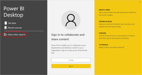
Illustration 2: Select Open Reports on the Splash Dialog that Appears
- Navigate to the file we downloaded.
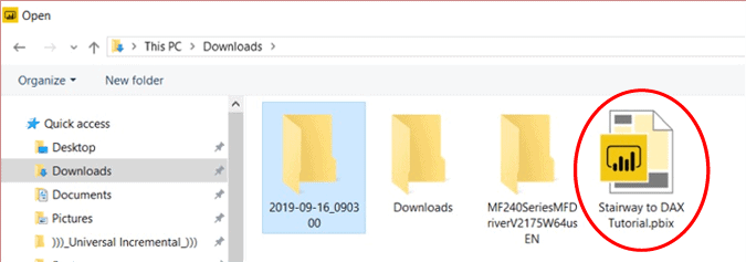
Illustration 3: Select the Stairway to DAX Tutorial File and Open …
- Click Open.
The .pbix file opens and we arrive within the Report view, which consists of a single tab containing a blank canvas. As many of us are aware, we can tell we are in the Report view because the current view (of the three views available, Report, Data, and Relationships, from top to bottom) is indicated by the yellow bar to the left of the icon.
- Click the Data and Relationship view icons along the left of Power BI Desktop, as desired, to become familiar with the sample model.
The DAX ALLSELECTED() Function
Introduction
According to the Data Analysis Expressions (DAX) Reference, the ALLSELECTED() function “removes context filters from columns and rows in the current query, while retaining all other context filters or explicit filters.” The Reference further states that ALLSELECTED() “gets the context that represents all rows and columns in the query, while keeping explicit filters and contexts other than row and column filters. This function can be used to obtain visual totals in queries.”
We will examine the syntax for the ALLSELECTED() function in this level, with a focus toward its use within simple visualizations. We’ll then undertake practice examples built around hypothetical business needs that illustrate typical uses for the function.
Discussion
ALLSELECTED(), as we have noted, supports “visual totals” via a measure. It can be particularly useful in instances where we want “% of (selected, or visual) totals,” as well, as we’ll see in the practice exercises. For a calculation containing ALLSELECTED() within, say, a matrix or table, the function removes only the filters created by the columns and rows of the visualization. All other filters are respected.
As a quick illustration, say we have a matrix that is presenting a column of values that represent total sales for each of its geographical locations for all time. The adjacent column is displaying total of all locations. Say that, adjacent to that column, we have a column containing a (highly popular) calculation that presents the percentage of the total contributed by each location to the total of the all calculations (numerator of the calculation is the total sales for each location, and denominator represents the total of all locations (in the middle column of the three described here).
Now, say we want to provide information consumers a means of “narrowing the presentation” of the visual, on the fly, to specific locations, say, within a given state / province. The contribution percent calculation we have constructed would present the calculation correctly for only the calculations shown (the locations we have selected via a slicer), but the “percentage of total” would remain the percent of each of the selected locations over the total for all locations, which may, indeed, be fine, depending upon the business requirement.
If we also wanted to see the percentage contribution to the total of selected (via the slicer) sections only, however, we would need to create a calculation that goes beyond a hard-coded total of all locations and allows the denominator, also, to flex to match the slicer selection and generate a total for the selected locations only. Using ALLSELECTED() within the calculation would make it possible to override the context of “all locations” to make desired “visual total” appear.
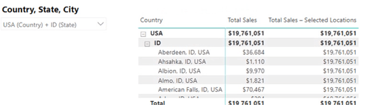
Illustration 4: ALLSELECTED() Supports “Visual Totals” via Slicers
So, to summarize, in Power BI, ALLSELECTED() in the calculation:
- Returns all the rows in a table / matrix visualization, or all the values in a column
- Removes context filters from columns and rows in the current measure / query
- Enforces filters that come from outside the visualization
Syntax
Syntactically, the parameters we provide are specified within the parentheses to the right of ALLSELECTED as shown:
ALLSELECTED([<tableName> | <columnName>[, <columnName>[, <columnName>[,…]]]] )
The two parameters are:
- tableName – (Optional) The name of an existing table, using standard DAX syntax. This parameter cannot be an expression.
- columnName – (Optional) The name of an existing column using standard DAX syntax, usually fully qualified. It cannot be an expression.
If there is one argument, the argument is either tableName or columnName. If there is more than one argument, they must be columns from the same table
Return Value and Further Remarks
ALLSELECTED() returns the context of the query without any column and row filters.
Moreover, ALLSELECTED() retains all filters explicitly set within the query, while retaining all context filters other than row and column filters.
Let's get some hands-on practice with ALLSELECTED() in the next section.
Practice
It’s time to get some exposure to what we’ve learned so far in this Level. To do so, we’ll put ALLSELECTED() to work within the definition of a few measures we add to our sample Power BI model within the Power BI Desktop. The intent, as in all the practice sessions of Stairway to DAX and Power BI, is to demonstrate the operation the function under examination in a straightforward, memorable manner. Let's move to the Power BI Desktop model we downloaded earlier as a platform within which to construct and execute the DAX we examine, and to view the results we obtain.
We’ll start with a simple business reporting need: The handful of colleagues with which we regularly work at a hypothetical client have expressed a keen interest in a “visual totals” capability similar to the one we outlined in our introductory discussion above: They want to be able to “narrow the presentation” of some of their visuals, based upon selection via slicer(s) that accompany the visuals. In particular, they want to focus, for purposes of a demo, on specific locations, say, within given cities. They wish to construct a “percentage of total” calculation such as we have described, where the values generated by the calculation flex to match the choice of cities made at runtime via a geographical slicer. The desired result: the percentage contributed by each city to the total sales of that selected group.
We examine the basic Power BI file they currently have, a sales and marketing model containing a small amount of data for retail merchandise over a few years, and determine upon a quick design to illustrate how we might meet this business need using the ALLSELECTED() function. We will use the “starter” model as it currently exists for the setup of a simple scenario that both meets the need and demonstrates the reason that ALLSELECTED() is required for this to happen. As a part of our efforts, we also provide a means by which the accuracy and completeness of the results we obtain are verified.
Create a Basic Reference Matrix to Support Verification of Practice Calculations
Let’s begin by building a basic matrix visualization to show simple totals across time. We will use this to help us verify that the values we deliver with our practice calculations are correct – a great habit to develop when developing solutions in the business environment.
- Ensure that we are in the Report view by clicking the top icon of the three located along the left edge of the window.
Illustration 5: Select the Report Icon …
- From the Fields pane, expand the Sales table, and drag the pre-existing Total Sales measure onto the blank canvas, as shown.
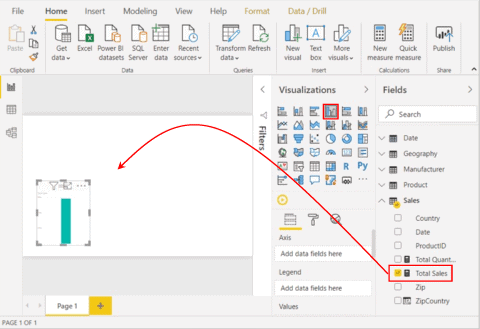
Illustration 6: Create a Placeholder Visualization with the Total Sales Measure
The default visualization is a Clustered Column Chart. Since this visualization will be used to present values for checking against calculations we create, let’s change it to a Matrix.
- With the new visualization selected, click the Matrix icon in the Visualizations pane.
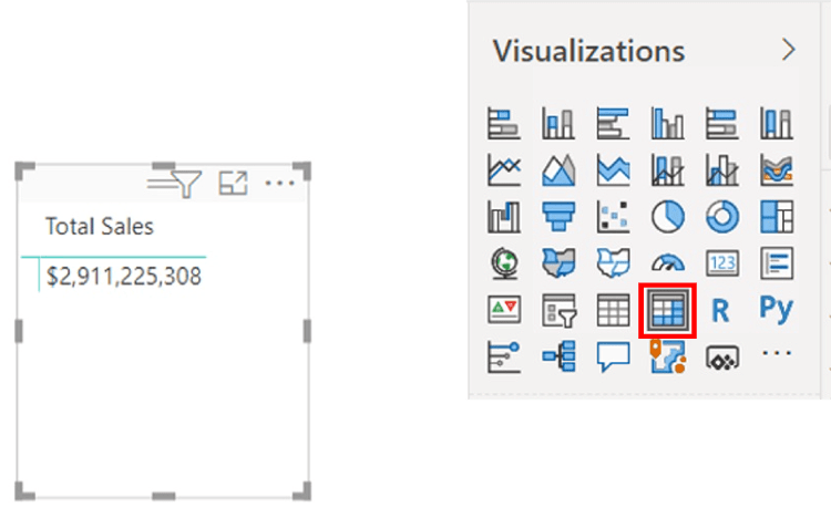
Illustration 7: Convert the Placeholder Visualization to a Matrix
Adjusting its position as we go, to keep it generally in the lower half of the page, let’s add some data to the new matrix.
- Ensure that the Fields button (the leftmost of the three), beneath the various visualization icons in the Visualizations pane, is selected.
- Drag the following data elements (‘Table’[Element]) from the Fields list into the indicated areas, in order:
Rows
- ‘Geography’[Country]
- ‘Geography’[State]
- ‘Geography’[City]
Columns
- ‘Date’[Year]
Values
- ‘Sales’[Total Sales] (already in place in the model)
The Fields tab of the Visualizations pane appears as shown:
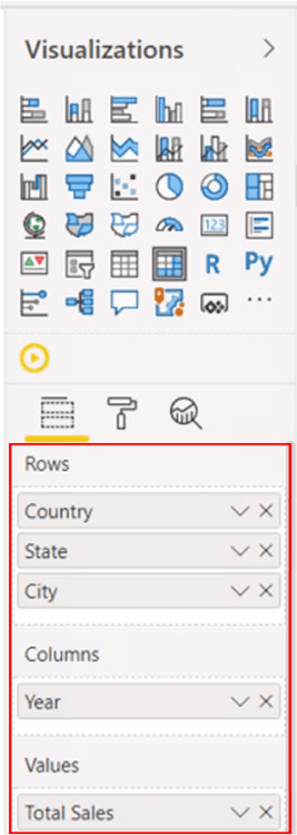
Illustration 8: Fields Tab for the Matrix, with Our Input
The new matrix appears as depicted, at this point:
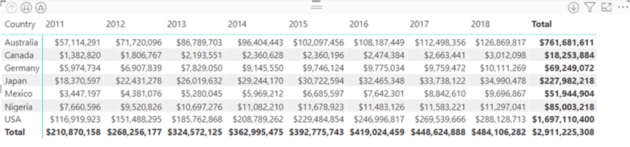
Illustration 9: Initial Draft of the Reference Matrix
We don’t need to spend too much time formatting this matrix – its sole purpose is to give us a breakdown of the data to support easy verification of the accuracy and completeness of the calculations that we will be creating. We can, however, take a few more steps to make it more useful (and efficient) in meeting its purpose.
- With the matrix selected, click the Format button (the middle of the three), beneath the visualization icons collection in the Visualizations pane.
- Expand the Row headers section by clicking the downward pointing caret button to the left of the title, as shown.
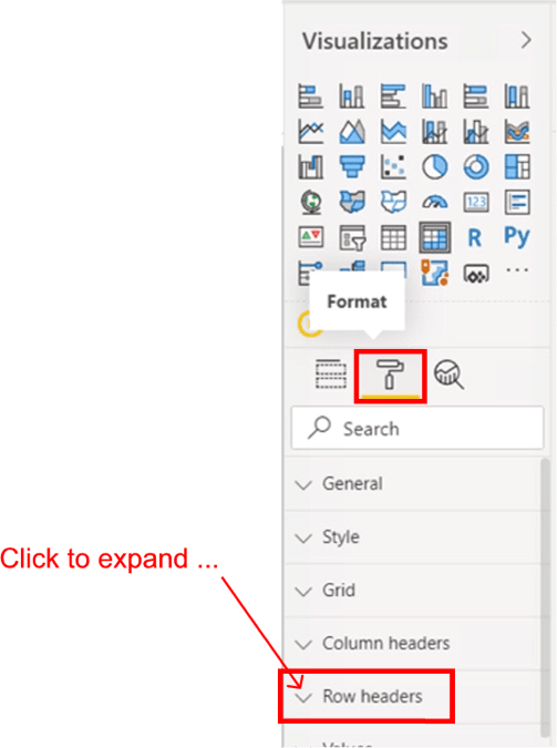
Illustration 10: Accessing Row Header Settings for the Matrix …
- Scroll toward the bottom of the settings within the expanded Row headers section and turn the setting, “+ / - icons,” to “On.”
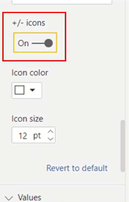
Illustration 11: Turn on the Visual Drilldown for the Matrix
A “+” sign appears to the left of the Row labels within the matrix, indicating that visual drilldown is enabled.
Next, let’s label the matrix we are creating – a minor point, but, as it will appear among other visualizations, it will be a good idea to note it for what it is: a reference tool for the report author.
- Click the now upward-pointing carat to the left of the Row headers section within which we have been working, to collapse the section.
- Scroll lower to the Title section of the Format settings.
- Click the Title slider to On.
- Expand by Title section by clicking the carat to the left of Title label.
- Type Reference Data in the Title text box.
- Set formatting as desired (you can see what I used in the illustration below).
The settings for the Title section of the Format tab appear as depicted.
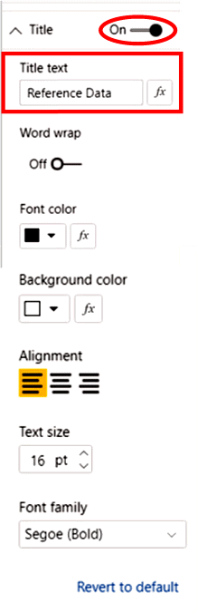
Illustration 12: Title Settings for the Reference Data Matrix
The new Reference Data matrix appears similar to that shown.
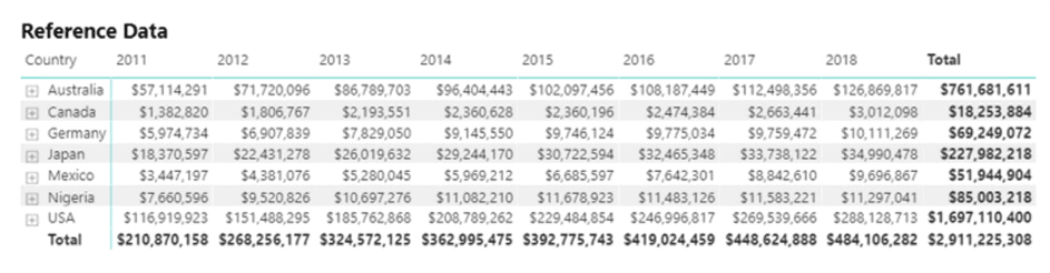
Illustration 13: The Reference Data Matrix with Modifications
We now have a means of checking values returned by calculations we are about to create using ALLSELECTED() and other functions. As I mention throughout the levels of Stairway to DAX and Power BI, having a means of verification like this for calculations we create with DAX is often helpful in providing quality solutions rapidly.
Add a Basic Slicer to the Canvas to Further Illustrate the Operation of ALLSELECTED()
Let’s add a slicer to the mix to make it easy to see how ALLSELECTED() works. We’ll place the slicer visualization in the left, upper corner of the canvas for easy access / visual confirmation of selections.
- Click on the blank area of the canvas in the upper left corner
- Click the Slicer icon in the Visualizations collection atop the Visualizations pane.
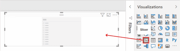
Illustration 14: Select the Slicer Visualization …
- Narrow the slicer toward the left upper corner to pre-position it.
- Expand the Geography table in the Fields pane, and add the following, in order, to the Field box of the Field tab underneath the Visualizations collection:
- Country
- State
- City
Our data field selection appears as shown within the slicer Field box:
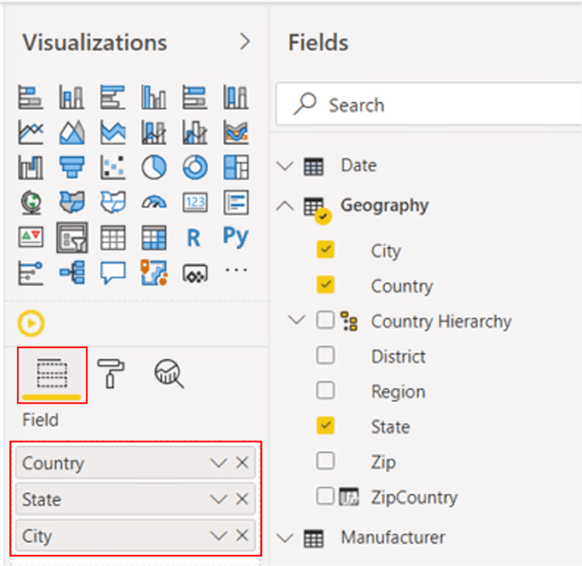
Illustration 15: Geography Fields Selected for the New Slicer …
- Move the mouse over the slicer, to the right of the “Country, State, City” label, until a couple of faint, gray symbols appear, as shown.
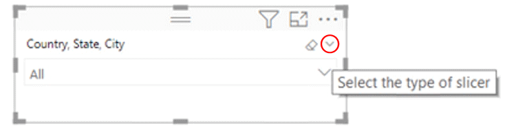
Illustration 16: Uncovering the Secretive Caret …
- Click the downward-pointing caret symbol to gain access to a choice of display options:
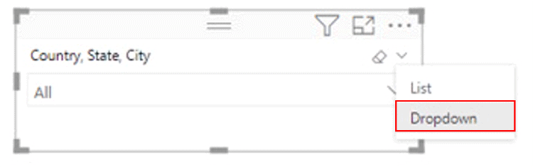
Illustration 17: Changing Slicer Selector Behavior to “Dropdown”
(I prefer Dropdown (versus a fixed list with checkboxes) for selector behavior, as it conserves real estate within canvas in general.)
- Click Dropdown here, if preferred.
- Back in the Format tab, Slicer header section, set formatting as desired.
The settings for the Slicer Header section of the Format tab for the new slicer appear similar to those depicted.
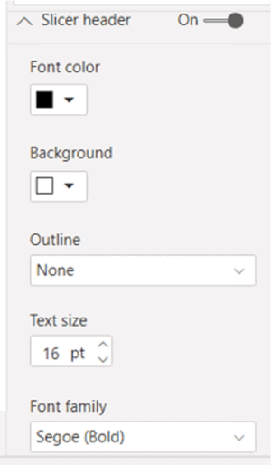
Illustration 18: Slicer Header Settings for the Geographical Slicer
The new Geography slicer appears, partially expanded, as shown.
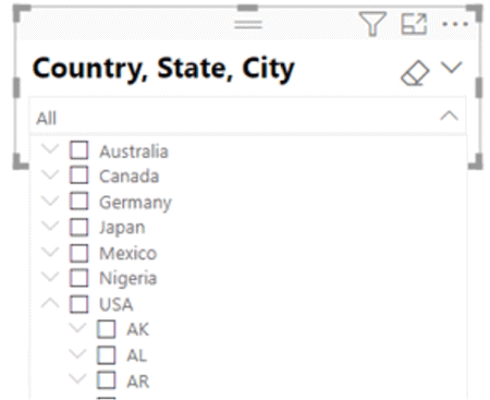
Illustration 19: The New Geography Slicer (Partially Expanded)
We’ll leave the new geographic slicer at “All” for now, and revisit it after we get the next measure in place.
Illustrate the Operation of ALLSELECTED() through Individual Measures We Create
We’re ready to get some exposure to the DAX ALLSELECTED() function. We’ll do this at a couple of levels, working within a matrix visualization that we’ll place above our Reference Data matrix for easy access.
Let’s create a simple scenario first, a matrix containing a sales total for all locations in the organization, which we’ll call “Worldwide Sales.” Our existing Total Sales measure should act as a great starting point, around which we’ll construct a matrix to house a few additional calculations we’ll put together to support a basic analysis that uses ALLSELECTED().
- Click the cursor on the canvas in the blank space to the right of the slicer that we have just created (above the Reference Data matrix).
- Click the matrix icon in the collection atop the Visualizations tab, to create a blank matrix on the canvas.
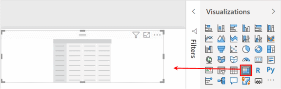
Illustration 20: Create a New Matrix on the Canvas
- From the Sales table within the Fields pane, add the pre-existing Total Sales measure to the matrix via the Values section of the Fields tab underneath the Visualizations collection.
This is the total of sales, for all locations, all time, etc. within the model.
- Using the steps we took in titling the matrix visualization we created above (we called it “Reference Data”), give this one the Title of “ST_SDAX015 – ALLSELECTED(),” (or any other title you choose), and format the values in the matrix as desired.
The new “starter matrix” appears as depicted.
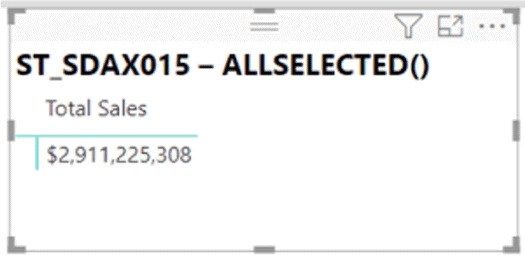
Illustration 21: The New Analysis Matrix Takes Shape …
- Ensuring that the above matrix visualization is selected, add the following to the Rows section of the Fields tab underneath the Visualizations collection:
- Country
- State
- City
The relevant portion of the Fields tab appears as shown.
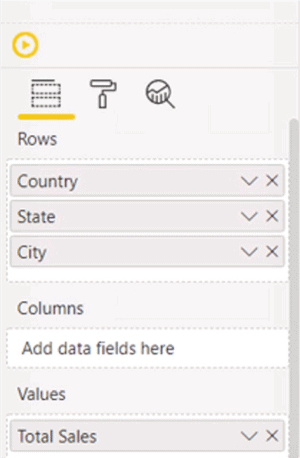
Illustration 22: New Row Additions in the Fields Tab
- Go to the Format tab for this matrix, and expand the Row headers section, as we did when creating the Reference Data matrix above.

Illustration 23: Adjusting Row Header Settings for the Matrix …
- Scroll toward the bottom of the settings within the expanded Row headers section and turn the setting, “+ / - icons,” to “On,” as we did for the first matrix above.
The “+” sign appears to the left of the Row labels within the matrix, indicating that visual drilldown is enabled. The new matrix visualization now appears, with a sample, partial drilldown, similar to the one shown.
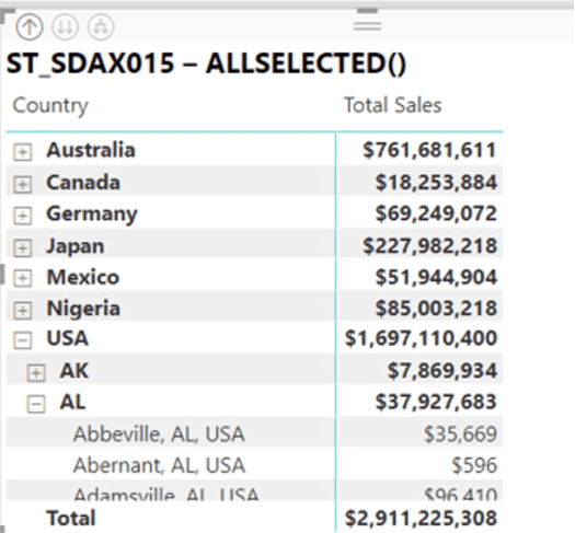
Illustration 24: Drill-down Capability in Place in the New Matrix
Next, let’s create some measures to gain an understanding of how ALLSELECTED() works.
Analysis 1: Employ ALLSELECTED() to Generate Selected Location Sales
Let’s build a simple analysis of the contribution of each of the selected sales locations of the organization to the total of selected locations. We already have Total Sales in place. Next, we’ll calculate the total for the aggregate of selected locations.
Create a measure called Total Sales – Selected Locations within the Sales table by taking the following steps:
- Click the ellipses ( “…” ) to the right of the Sales table within the Fields pane.
- Click New Measure atop the context menu that appears, as shown.
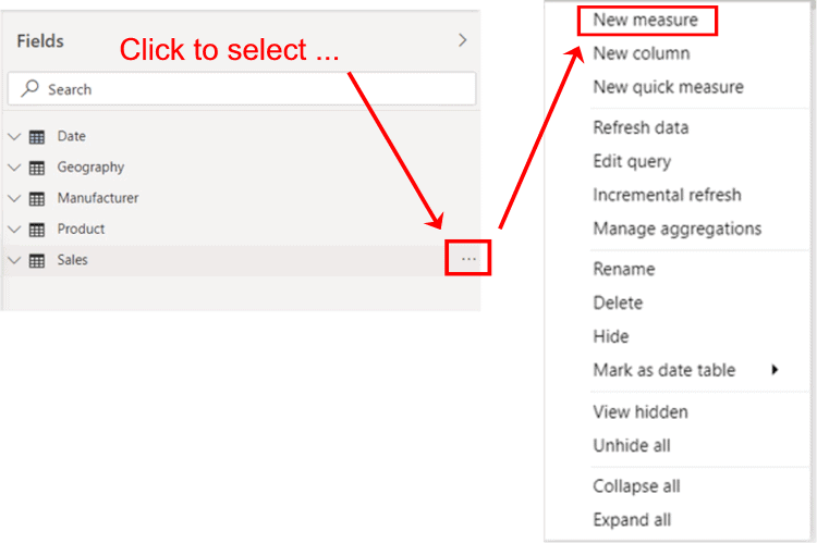
Illustration 25: Click New measure to Begin Design …
- Type the following into the Formula bar for the new measure that appears:
Total Sales – Selected Locations =
CALCULATE(
[Total Sales], ALLSELECTED(Geography))
- Click the check mark icon on the left side of the Formula bar to commit the new measure.

Illustration 26: Commit the New Measure …
We employ the ALLSELECTED() function, within the CALCULATE() function, to “re-contextualize” the Total Sales value to “Total Sales for the selected locations.”
NOTE: For an introduction to the DAX CALCULATE() function, see Stairway to DAX and Power BI - Level 14: DAX CALCULATE() Function: The Basics
EDITOR: At the time of writing, Level 14 was in the queue for publication. Can we please add a link to that article (reference highlighted above) when publishing this one? THANKS!
- Ensuring that the new measure is still selected within the Sales table, and in the Measure tools tab of the toolbar, format it as “Currency,” zero decimal places.
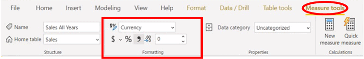
Illustration 27: Format the New Measure – Rounded Currency
Now, let’s pull the new measure into the matrix.
- Add the new Total Sales – Selected Locations measure to the matrix via the Values section of the Fields tab underneath the Visualizations collection.
The new matrix appears, thus far, as depicted.
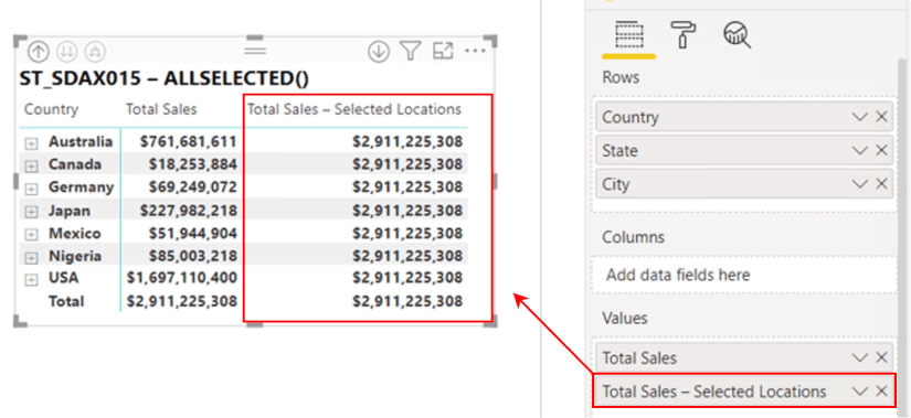
Illustration 28: New Visual with Measure Containing ALLSELECTED()
We can easily verify that the accuracy of this unfiltered total, for all locations (and for all years, etc.), using our Reference Data matrix.
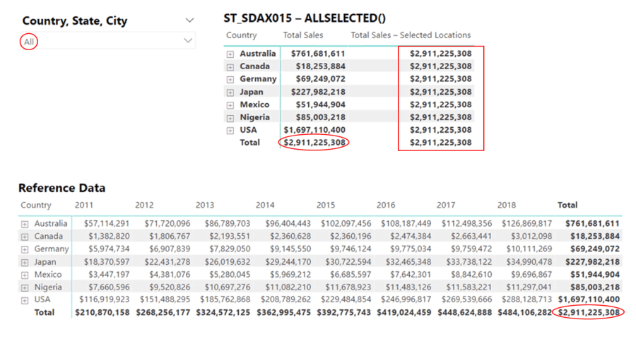
Illustration 29: Verifying Total Sales – Selected Locations with No Filters Applied
Now, since we have three visualizations in place, it might be a good time to make one small adjustment to ensure the “independence” of our Reference Data matrix. Since we are using it to ascertain accuracy / completeness of values created through the interaction of the slicer and the ST_SDAX015 – ALLSELECTED() matrix, let’s adjust the default interaction that exists between the three visualizations at the current juncture.
- Click the Country, Sate, City slicer, to select it.
- Click the Format tab on the toolbar atop Power BI Desktop.
- Click Edit interactions in the upper left corner of the tab.
- Ensure that interaction remains “on” for the ST_SDAX015 – ALLSELECTED() matrix (the default of left button selected) and “off” (the circle with a downward slash button) for the Reference Data matrix, as depicted.
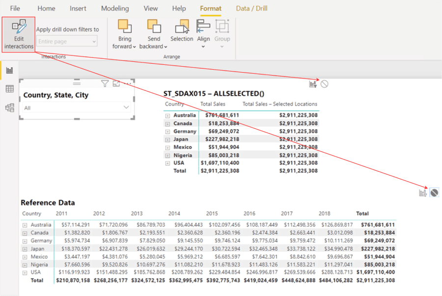
Illustration 30: Turning Off Interaction between Slicer and Reference Data Matrix
Going forward, the Reference Data matrix will come back with all locations, instead of filtering for our slicer selection, as does the ST_SDAX015 – ALLSELECTED() matrix.
Let’s check out the interaction of the slicer.
- Select “ID” (USA state of Idaho) in the Country, State, City slicer, as shown.
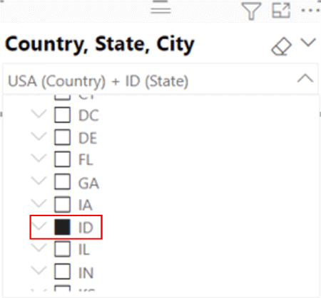
Illustration 31: Narrowing the Selection to a Single U.S. State (Idaho), via the Slicer
We should be able to notice, at this point, that the slicer filter appears to interact only with the upper matrix, leaving the Reference Data matrix at default of “all countries.” (Collapse the State of ID within the dropdown selector of the slicer to replicate the illustration below.)
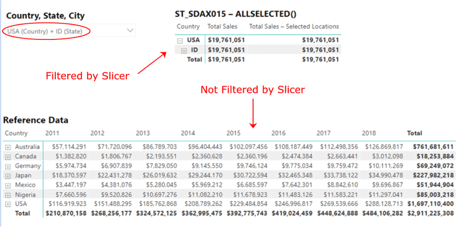
Illustration 32: Slicer Filters the Upper Matrix Only
We can also witness the action of the ALLSELECTED() function, within the CALCULATE() function, to re-contextualize” the Total Sales value to “Total Sales for the selected locations” within the Total Sales – Selected Locations measure we created to demonstrate this operation of the function. Finally, we can ascertain accuracy of the value returned by that measure by verifying the Total value for Idaho within the Reference Data matrix below, as depicted.
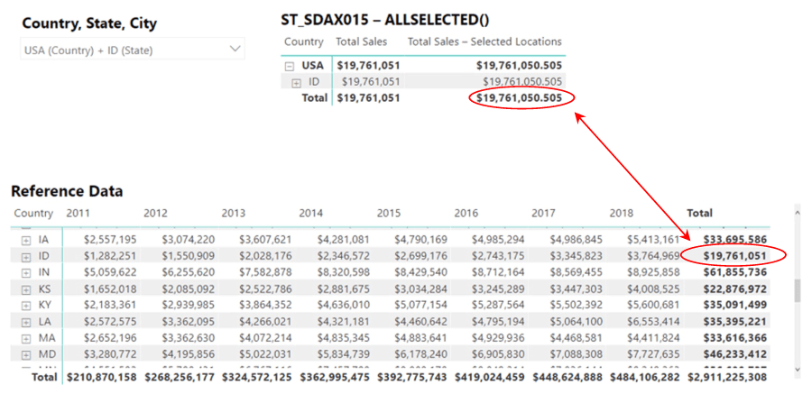
Illustration 33: Slicer Filters the Upper Matrix Only
When we drill down upon the state of Idaho in this instance, the Total Sales measure gives us the total for the cities upon which we drill, while the Total Sales – Selected Locations measure renders the Total of all the selected locations on every row. Let’s limit the size of that selection in the immediate scenario of Idaho, within which the client makes sales to customers in many cities / towns.
- Click the ST_SDAX015 – ALLSELECTED() matrix to select it.
- In the slicer, click the “eraser” icon (in the pair of light gray icons to the right of the Country, State, City label in the slicer header) to clear all slicer headings (often easier than turning them off individually, etc.)
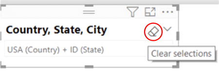
Illustration 34: Clearing All Slicer Selections …
- Within USA, again, make the following three ID city selections within the slicer (hold down CTRL to multi-select):
- Idaho Falls
- Inkom
- Pocatello
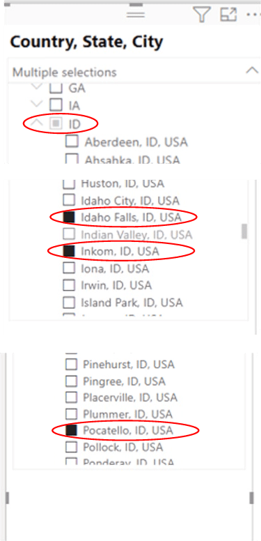
Illustration 35: Select Three Idaho Cities in the Slicer
- Within the ST_SDAX015 – ALLSELECTED() matrix, expand ID to expose the three selected cities, as shown.
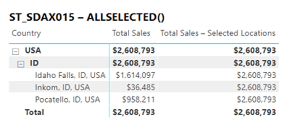
Illustration 36: The Selected Cities Appear …
We see the Total Sales value flexes to accommodate the three selected cities. We note, too, that the Total Sales – Selected Locations remains the total of the entire selection, as expected.
Let’s extend our sales analysis a bit by adding a measure to calculate percentage of contribution of each member of a selection to the total of the members in that selection (Idaho in our geographical example), and then finally touch upon how the ALL() function can be called upon to add even more analytical utility to the matrix.
Analysis 2: Employ ALLSELECTED() to Generate Selected Location Sales Contribution Percent
Having generated a column containing Total Sales of each of the selected locations within the analysis we are building within the new ST_SDAX015 – ALLSELECTED() matrix, we next want to add a measure that presents each location’s percentage contribution to the grand total of the selected locations’ group sales. As was the case with the first measure we added to our analysis, using the ALLSELECTED() function within this measure will make it return results based upon our slicer selection.
- Create a new measure called % Total Selected Locations within the Sales table:
Formula:
% Total Selected Locations =
DIVIDE([Total Sales], [Total Sales – Selected Locations])
Format:
Percent (%), 1 decimal place
- Click the check mark icon on the left side of the Formula bar to commit the new measure.
Here, our objective is to divide Total Sales for each city for by the total of all selected cities. In this case, each of the three cities we selected in Idaho by the total sales of the combined three cities.
While we might have simply used the “/” character to perform the division, the DIVIDE() function comes in handy in many instances, as it manages division by zero for us. It performs division, and returns either a BLANK() upon division by zero, or an alternate result that we specify.
NOTE: The measure we have just constructed works fine in the current situation, where we happen to be using the Total Sales – Selected Locations measure separately in our analysis, so we can visually ascertain that the percentages returned appear to be correct mathematically. Had we chosen to do so, obviously, we might have performed the % Total Selected Locations calculation in a single, combined measure, which would have looked like this:
% Total Selected Locations =
DIVIDE([Total Sales], CALCULATE([Total Sales], ALLSELECTED(Geography)))
- Select the ST_SDAX015 – ALLSELECTED() matrix visualization, and add the new % Total Selected Locations measure to the Values section of the Fields tab for the matrix, between the existing Total Sales and Total Sales – Selected Locations measures, as depicted.
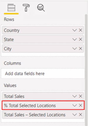
Illustration 37: % Total Selected Locations Added to Values in the Fields Tab
The matrix appears, with the latest addition, as shown.
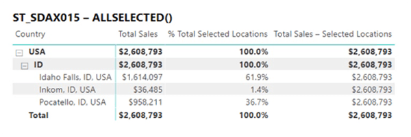
Illustration 38: % Total Selected Locations Measure in Place in the Matrix
Next, let’s expand our focused analysis of contribution to sales to reflect the additional insight of contribution by each of the selected locations to the overall international sales totals.
Analysis 3: Revisit the use of ALL() in Another Measure to Extend the Utility of the Visualization
We introduced the DAX ALL() function in Level 14 of the Stairway to DAX and Power BI. Let’s leverage the capabilities we examined in that function to extend our analysis of contribution to sales totals by location here. Having created a matrix to contain the logic needed to present a view of the sales of each of a group of selected locations, as well as the percentage contribution by each of the member locations to the total sales of the selected group, let’s add another pair of measures to return the total worldwide sales value and the percentage contribution of each of the selected locations to the worldwide total.
EDITOR: At the time of writing, Level 14 was in the queue for publication. Can we please add a link to that article (reference highlighted above) when publishing this one? THANKS!
- Create a new measure called Total Sales - Worldwide within the Sales table:
Formula:
Total Sales - Worldwide =
CALCULATE([Total Sales], ALL(Geography))
Format:
Currency, 0 decimal places
- Click the check mark icon on the left side of the Formula bar to commit the new measure.
Here, we are re-setting context for Total Sales (all years) to “All Geography,” or all sales locations. We are simply creating a denominator for another “Percentage of Total” calculation – the denominator this time representing all sales locations versus the locations upon which we are focusing in our analysis.
NOTE: For an introduction to the DAX ALL() function, see Stairway to DAX and Power BI - Level 13: Simple Context Manipulation: Introducing the DAX All() Function.
- Select the ST_SDAX015 – ALLSELECTED() matrix visualization, and add the Total Sales - Worldwide measure to the Values section of the Fields tab for the matrix, as depicted.
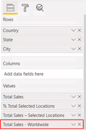
Illustration 39: Total Sales – Worldwide in Place in the Matrix
Finally, we’ll add the % Total Sales Worldwide measure to complete our analysis for the time being.
- Create a new measure called % Total Sales - Worldwide within the Sales table:
Formula:
% Total Sales - Worldwide =
DIVIDE([Total Sales], [Total Sales - Worldwide])
Format:
Percent
- Click the check mark icon on the left side of the Formula bar to commit the new measure.
We now have a measure that delivers the percentage of all sales worldwide that is contributed by each member of our selection within the slicer.
- Select the ST_SDAX015 – ALLSELECTED() matrix visualization, once again, and add the % Total Sales - Worldwide measure to the Values section of the Fields tab for the matrix, between the existing Total Sales – Selected Locations and Total Sales - Worldwide measures, as shown.
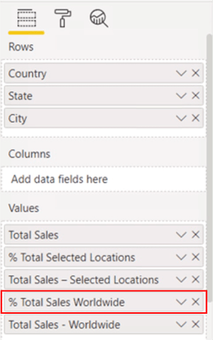
Illustration 40: % Total Sales – Worldwide in Place in the Matrix
The analysis matrix appears, with the latest additions, as shown.
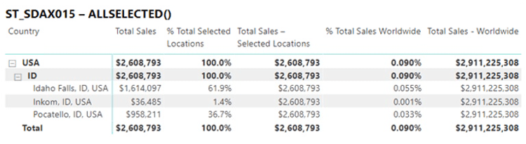
Illustration 42: % Total Sales Worldwide and Total Sales Worldwide Measures in the Matrix
We now have a basic visualization that can help information consumers begin to analyze the contribution of individual sales geographies to total sales – totals both for the entire organization and for the composite groups we can select at runtime. In reality, of course, we may not need to display, in the visualization, the Total Sales measures that serve as denominators in the percentage calculations we created – this is merely a way of demonstrating the role these values play in reaching the desired ends (as well as making it easy to independently our percentage calculations). Much more could be also be added to the analysis, of course, including an analysis of the change of the contribution percentages over time, analysis of external factors that may affect the individual geographies, such as economic conditions and demographic factors, and other analytical considerations.
I hope that the simple exercises we have explored in this Level have introduced the operation of DAX ALLSELECTED() function in a way that encourages its use in delivering great analysis insight within the business environment. Opportunities to employ ALLSELECTED() will no doubt appear regularly as we face the requirements of our clients and employers to meet reporting and analysis needs, particularly where run-time slicing / parameterization is a factor.
Summary
In this Level of Stairway to DAX and Power BI, we exposed the DAX ALLSELECTED() function. We discussed the general purposes and operation of ALLSELECTED(), and then focused upon putting it to work in the removal of context filters from columns and rows within a given query, while leaving remaining context or explicit filters in place. As part of our discussion, we examined the syntax involved with using ALLSELECTED(), and then constructed basic, illustrative examples of uses of the function in practice exercises. Finally, for each example we undertook, we explored the results datasets we obtained.
This article is part of the parent Stairway to DAX and Power BI.