
In this Level, we will introduce the powerful DAX CALCULATE() function. As we become more familiar with using DAX in Power BI, we reach an appreciation for its versatility and usefulness. CALCULATE() can be employed in a wide array of scenarios in Power BI, enforcing filters that range in complexity from very simple to advanced. It enables us to manipulate the context within which a measure is evaluated both easily and efficiently, so that, regardless of which axes are selected and / or filters are employed within our reports, the filter specifications that we feed to CALCULATE() are applied.
We’ll introduce CALCULATE() within the setting of some of its simpler uses. As we progress through the Stairway to DAX and Power BI, we will employ CALCULATE() many times, where it will add sophistication and efficiencies to our measures and, consequently, to the visualizations those measures support. Our focus in this Level will be the use of CALCULATE() with simple filters.
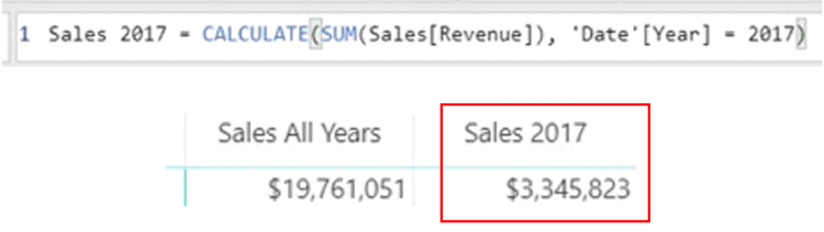
Illustration 1: Introducing CALCULATE() with Simple Filters
As a part of our exploration, we will examine how CALCULATE() can be employed to alter context, to achieve results similar to the kinds of things we might need to generate for clients or employers in our own environments. As a part of our introduction, we will examine the output we obtain, employing CALCULATE() via measures we construct within a Power BI model in the practice session that follows. We’ll discuss the purpose of the function, and how to use it with basic filters, while looking beyond basic filters a little to generate appreciation for additional capabilities of the function.
During our exploration of the CALCULATE() function, we will:
- Examine the syntax involved in exploiting the function;
- Undertake illustrative examples of the uses of the function in practice exercises;
- Briefly discuss the results datasets we obtain in each of the practice examples.
Preparation for the Practice Exercises in this Level
Assuming that you have installed Power BI Desktop (the illustrations in this Level reflect the June 2020 release), you are ready to download and open the sample Power BI Desktop file that we will use for hands-on practice with the concepts we introduce.
NOTE: The latest version of Power BI is available for free download at www.powerbi.com.
Download Sample Power BI File (.pbix) for Use in this Level
The sample Power BI file we’ll be using contains fully imported data, and a few pre-existing calculations that might be helpful in general. We will add the calculations or visuals upon which we focus in this Level as we go. Using the sample dataset we provide will ensure that the results you obtain in following the detailed steps of the exercises agree to the results we obtain (and depict) as we progress.
Once the sample .pbix file is downloaded, take the following steps to open it in Power BI Desktop.
- Open Power BI Desktop.
- Select File - Open other reports from the splash dialog that appears upon entry, as shown.
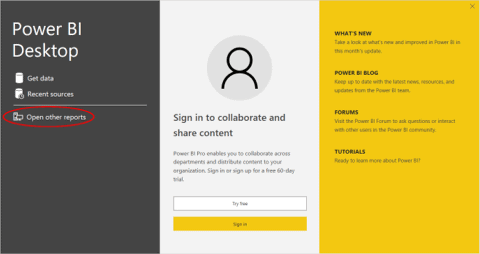
Illustration 2: Select Open Reports on the Splash Dialog that Appears
- Navigate to the file we downloaded.
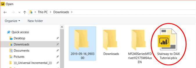
Illustration 3: Select the Stairway to DAX Sample and Open …
- Click Open.
The .pbix file opens and we arrive within the Report view, which consists of a single tab containing a blank canvas. As many of us are aware, we can tell we are in the Report view because the current view (of the three views available, Report, Data, and Relationships, from top to bottom) is indicated by the yellow bar to the left of the icon.
- Click the Data and Relationship view icons along the left of Power BI Desktop, as desired, to become familiar with the sample model.
The DAX CALCULATE() Function
Introduction
According to the Data Analysis Expressions (DAX) Reference, the CALCULATE() function “evaluates an expression in a context that is modified by the specified filters.” CALCULATE() is an oft-used function within Power BI, as it supports the sometimes complex calculations we need to perform the data analysis and reporting needs we encounter in the business environment.
We will examine the syntax for the CALCULATE() function in this level, with a focus toward its use with simple filters. We’ll then undertake practice examples built around hypothetical business needs that illustrate logical uses for the function.
Discussion
CALCULATE(), as we have noted, serves as a means of executing an expression within a modified filter context. It involves two parameters:
- Expression – The expression to be evaluated
- Filter – (Optional) A comma-separated list of Boolean expression(s) or table expressions(s) that define a filter
Syntax
Syntactically, the parameters we provide are specified within the parentheses to the right of CALCULATE as shown:
CALCULATE(<expression>,<filter1>,<filter2>…)
In cases where the requirement might be to filter the expression by more than one condition, we can add multiple filters, separated by commas, to the function.
The expression used as the first parameter is essentially the same as a measure (aggregation, calculation, etc.). A Boolean expression used as an argument can contain any function that looks up a single value, or that calculates a scalar value, but:
- Cannot reference a measure
- Cannot use a nested CALCULATE() function
- Cannot use any function that scans or returns a table, including aggregation functions
Return Value and Further Remarks
CALCULATE() returns the result of the expression evaluated in the specified filter context.
While we are focusing primarily upon basic filter arguments in this Level, we focus in other Levels upon how filter arguments can be used in additional ways, including:
- Filter removal
- Filter restoration
- Via table expressions
Let's get some hands-on practice with CALCULATE() in the next section.
Practice
To reinforce our understanding of the basics we've covered so far, we will follow our typical pattern of employing the function under examination in this Level within the definition of some calculations. We'll work with CALCULATE() via a few measures we add to our sample Power BI model within the Power BI Desktop. Moreover, we will examine the use of CALCULATE() in combination with another function (a practice we’ll see often in working with CALCULATE() in other Levels). The intent, as in all the practice sessions of the Stairway to DAX and Power BI series, is to demonstrate the operation of each of the functions we examine in a straightforward, memorable manner.
Note: Keep in mind that CALCULATE(), and the surrounding concepts of evaluation context and context transition themselves, can get into advanced topics that may require significant study and exposure to master. Our purpose here is to introduce CALCULATE() and its use enough to bring it to bear within subsequent Levels of the Stairway to DAX and Power BI. We will expose more of the utility and sophistication that the function can offer as we encounter needs for it in our continuing exploration of DAX.
Let's move to the Power BI Desktop model we downloaded earlier as a platform within which to construct and execute the DAX we examine, and to view the results we obtain. We’ll start with a simple business reporting need: Although only a few colleagues at a hypothetical client seem to understand the concept of context within DAX, a group with whom we are doing some prototyping work have asked us to demonstrate how they can take their calculations to the next level, and become able to style calculations that “flex” with change of context. Some have heard of the CALCULATE() function, and just want to see example measures that employ CALCULATE().
We examine the basic model they currently have, a sales and marketing model containing a small amount of data for retail merchandise over a few years. The engagement team objective has recently been to begin prototyping with Power BI Desktop, to replicate what they have been delivering via the reporting and analysis tools they already have. We will use the “starter” model as it currently exists, and get underway with demonstrating the function as requested.
Create a Basic QA Matrix to Support Verification of Practice Calculations
Let’s begin by building a basic matrix visualization to show simple totals across time. We will use this to help us verify that the values we deliver with our practice calculations are correct – a great habit to develop when developing solutions in the business environment.
- Ensure that we are in the Report view by clicking the top icon of the three located along the left edge of the window.
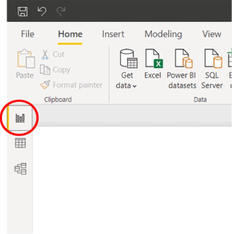
Illustration 4: Select the Report Icon …
- From the Fields pane, expand the Sales table, and drag the pre-existing Total Sales measure onto the blank canvas, as shown.
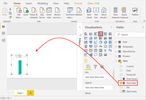
Illustration 5: Create a Placeholder Visualization with the Total Sales Measure
The default visualization is a Clustered Column Chart. Since this visualization will be used to present values for checking against calculations we create, let’s change it to a Matrix.
- With the new visualization selected, click the Matrix icon in the Visualizations pane.
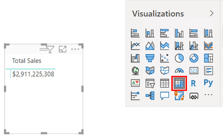
Illustration 6: Convert the Placeholder Visualization to a Matrix
Adjusting its position as we go, to keep it generally in the lower half of the page, let’s add some data to the new matrix.
- Ensure that the Fields button (the leftmost of the three), beneath the various visualization icons in the Visualizations pane, is selected.
- Drag the following data elements (‘Table’[Element]) from the Fields list into the indicated areas, in order:
Rows
- ‘Geography’[State]
- ‘Geography’[City]
- ‘Product’[Category]
Columns
- ‘Date’[Year]
Values
- ‘Sales’[Total Sales] (already in place in the model)
The Fields tab of the Visualizations pane appears as shown:
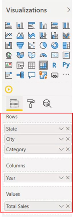
Illustration 7: Fields Tab for the Matrix, with Our Input
The new matrix appears as depicted, at this point:
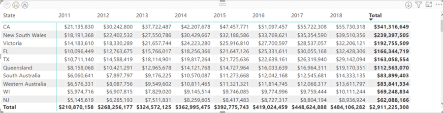
Illustration 8: Initial Draft of the Reference Matrix
We don’t need to spend too much time formatting this matrix – its sole purpose is to give us a breakdown of the data to support easy verification of the accuracy and completeness of the calculations that we will be creating. We can, however, take a few more steps to make it more useful (and efficient) to that end.
- Within the Filters pane, Filters on this visual section, set the State to “ID” (Idaho) for the matrix, as depicted. (We’re doing this mainly to limit scrolling, etc., in the matrix for some of the steps we perform in this Level.)
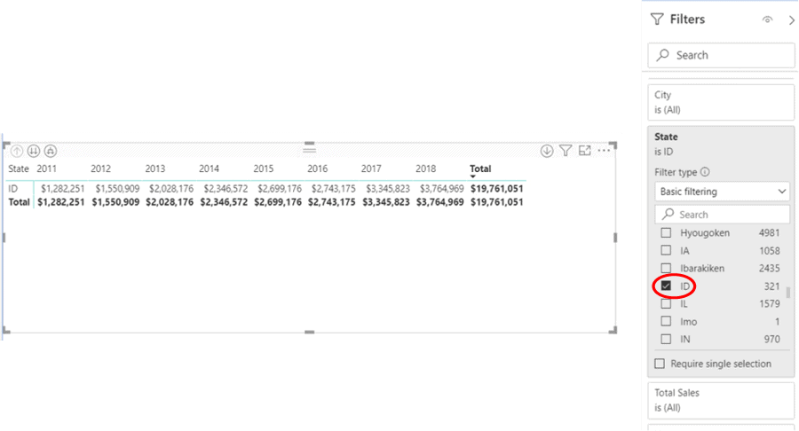
Illustration 9: The Reference Matrix So Far …
- With the matrix selected, click the Format button (the middle of the three), beneath the visualization icons collection in the Visualizations pane.
- Expand the Row headers section by clicking the downward pointing caret button to the left of the title, as shown.
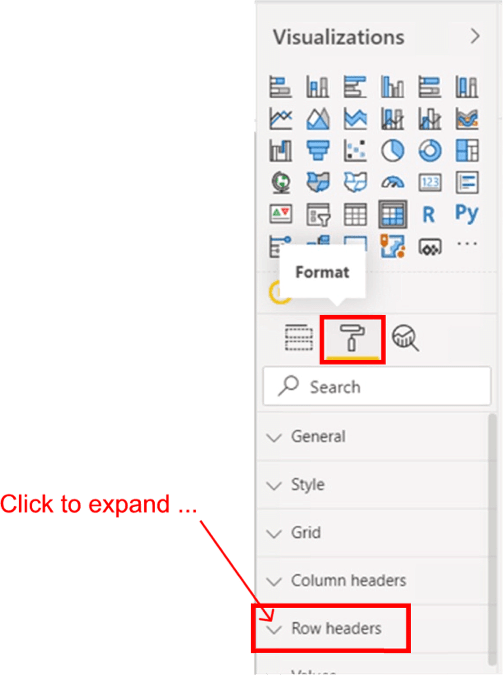
Illustration 10: Adjusting Row Header Settings for the Matrix …
- Scroll toward the bottom of the settings within the expanded Row headers section and turn the setting, “+ / - icons,” to “On.”
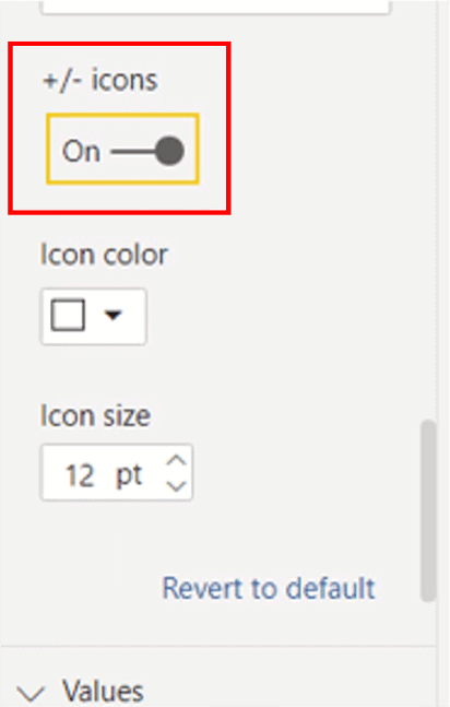
Illustration 11: Turn on the Visual Drilldown for the Matrix
The “+” sign appears to the left of the Row labels within the matrix, indicating that visual drilldown is enabled.
Next, let’s label the matrix we are creating – a minor point, but, as it will appear among other visualizations, it will be a good idea to note it for what it is: a reference tool for the report author.
- Click the now upward-pointing carat to the left of the Row headers section within which we have been working, to collapse the section.
- Scroll lower to the Title section of the Format settings.
- Click the Title slider to On.
- Expand by Title section by clicking the carat to the left of Title label.
- Type Reference Data in the Title text box.
- Set formatting as desired (you can see what I used in the illustration below).
The settings for the Title section of the Format tab appear as depicted.
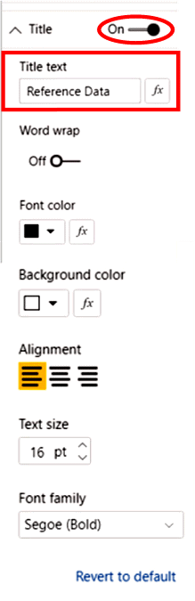
Illustration 12: Title Settings for the Reference Data Matrix
- Click the “+”” sign to the left of “ID” in the leftmost (“State”) column of the matrix.
- If necessary, sort the Idaho cities that appear, A-to-Z, by clicking the upward pointing (“ascending”) caret within the State column label (the caret appears when we mouse over the column label), as depicted.
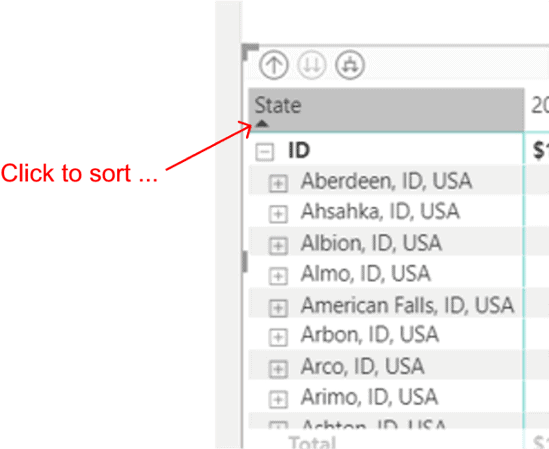
Illustration 13: Sort Idaho Cities A-to-Z …
- Scroll to the city of Pocatello (“Pocatello, ID, USA”), and click the “+” sign to its left, to expose the product categories sold there.
The Pocatello excerpt of the matrix appears as shown.
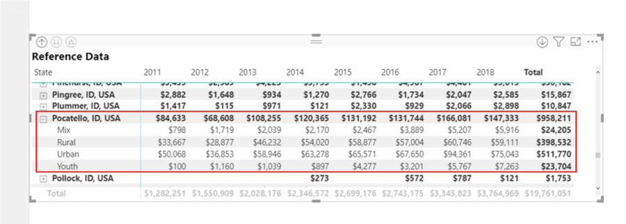
Illustration 14: View of the City/Category Drilldown at this Point …
We now have a means of checking some of the values returned by a few calculations we are about to create using CALCULATE(). As I mention here as well as in other Levels of the Stairway to DAX and Power BI, having a point of verification like this for calculations we create with DAX is often helpful in providing quality solutions rapidly.
Illustrate the Operation of CALCULATE() through Individual Measures We Create
We’re ready to get some exposure to the DAX CALCULATE() function. We’ll do this at a couple of levels, working with a matrix visualization that we’ll place above our Reference Data matrix for easy access.
Example 1: CALCULATE() Contains a Measure with No Filters
Create a measure called Sales All Years within the Sales table by taking the following steps:
- Click the ellipses ( “…” ) to the right of the Sales table within the Fields pane.
- Click New Measure atop the context menu that appears, as shown.
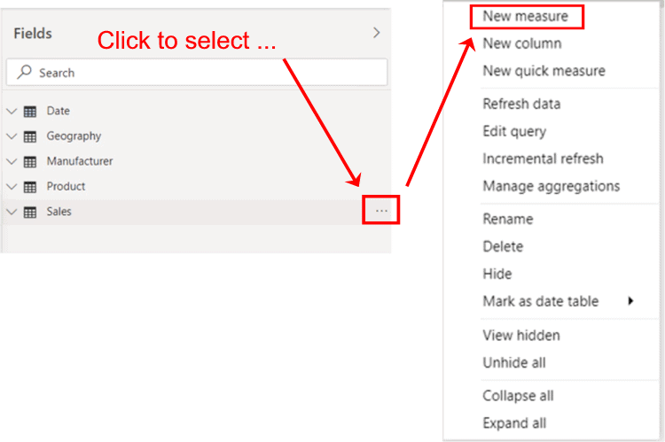
Illustration 15: Click New measure to begin design …
- Type the following into the Formula bar for the new measure that appears:
Sales All Years = CALCULATE([Total Sales])
- Click the check mark icon on the left side of the Formula bar to commit the new measure.

Illustration 16: Commit the New Measure …
Note that this is about as simple as it gets with CALCULATE(): A measure consisting of the CALCULATE() function containing merely another simple measure. My point is to illustrate that, with no additional filters imposed, the original calculation returns the same result as we would see the internal measure, Total Sales, return.
- Ensuring that the new measure is still selected within the Sales table, and in the Measure tools tab of the toolbar, format it as “Currency,” zero decimal places.
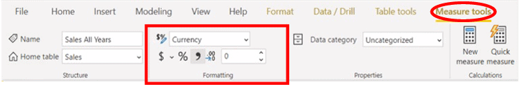
Illustration 17: Format the New Measure – Rounded Currency
Now, let’s create a new matrix within which we can home this new calculation, together with those that follow it.
- Click the cursor on the canvas in the blank space above the matrix visualization we have just created.
- Click the matrix icon in the collection atop the Visualizations tab, to create a blank matrix on the canvas.
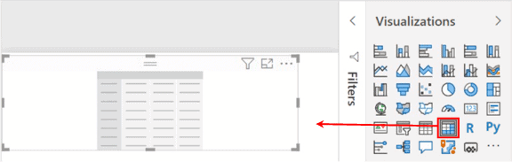
Illustration 18: Create a New Matrix on the Canvas
- Add the new Sales All Years measure to the matrix via the Values section of the Fields tab underneath the Visualizations collection.
- Set a visual-level filter of “State is ID,” to keep the sizes in control.
- Using the steps above for titling the matrix visual, give this one the Title of “CALCULATE() Examples,” and format the values in the matrix as desired.
The new matrix appears, thus far, as depicted.
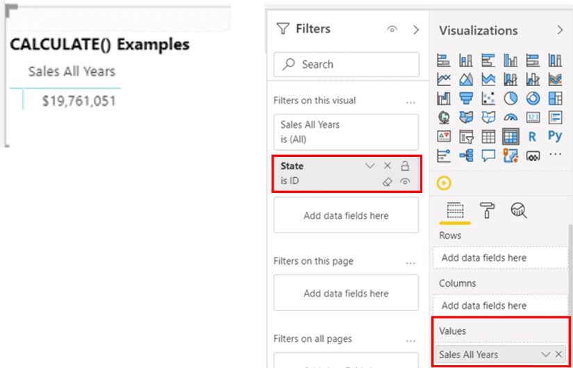
Illustration 19: New Visual with Measure containing CALCULATE()
Let’s move into some examples where we perform basic filtering via the CALCULATE() function.
Example 2: CALCULATE() Contains a Measure with a Single Filter
- Create a new measure called Sales 2017 within the Sales table:
Formula:
Sales 2017 = CALCULATE(SUM(Sales[Revenue]), 'Date'[Year] = 2017)
Format:
Currency, 0 decimal places
- Click the check mark icon on the left side of the Formula bar to commit the new measure.
Here, we are filtering sales by year 2017 (Date table).
- Select the CALCULATE() Examples matrix visualization, and add the Sales 2017 measure to the Values section of the Fields tab for the matrix (underneath the Total Sales value we added earlier), as shown.
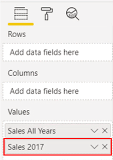
Illustration 20: New Measure Sales 2017 Added to Values in the Fields Tab
The matrix appears, with the new addition, as shown. The value of the Sales 2017 measure agrees with the value for the full state of Idaho for 2017, per the reference matrix, as shown.
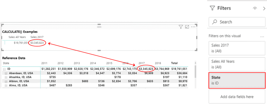
Illustration 21: Sales 2017 Agreed to 2017 Sales for Idaho in Reference Data
Let’s take a look at another simple, single filter scenario with CALCULATE().
Example 3: CALCULATE() Contains a Measure with Different Single Filter
This time, we’ll work with another table in the model, the Geography table, from the perspective of filtering. Say we want to focus on total sales for a single, tiny town in Idaho. We’d like to return total sales for the town of Inkom.
- Create a new measure called Total Sales-Inkom, ID within the Sales table:
Formula:
Total Sales-Inkom, ID =
CALCULATE([Total Sales], Geography[City]="Inkom, ID, USA")
Format:
Currency, 0 decimal places
- Click the check mark icon on the left side of the Formula bar to commit the new measure.
Here, we are filtering total sales – for all years of the model – for those achieved in Inkom.
- Select the CALCULATE() Examples matrix visualization, and add the Total Sales-Inkom, ID measure to the Values section of the Fields tab for the matrix (underneath the Sales - 2017 value we added earlier), as depicted.
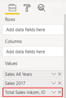
Illustration 22: Total Sales-Inkom, ID Added to Values in the Fields Tab
The matrix appears, with the latest addition, as shown. As expected, the value of the Total Sales-Inkom, ID measure agrees with the value for the total (all years) sales for Inkom, ID, USA, according to the reference matrix, as shown.
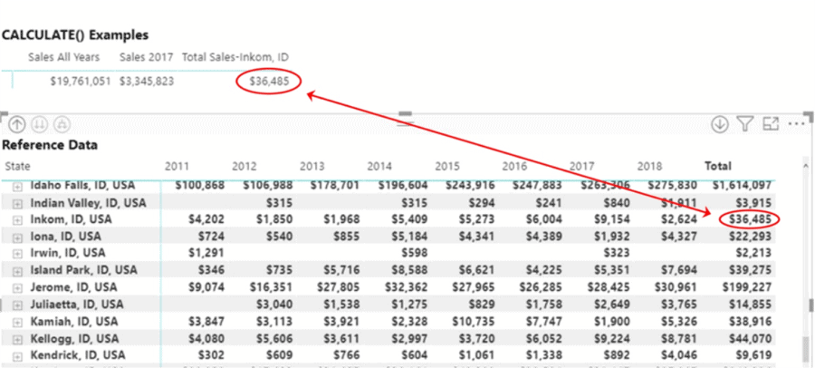
Illustration 23: All Years’ Total Sales-Inkom, ID, Agrees to Total Sales for Inkom, Idaho in Reference Data
Next, let’s use filters from multiple tables within the CALCULATE() function to pinpoint an even more narrowed balance.
Example 4: CALCULATE() Contains a Measure Filtered across Multiple Tables
Next, we’ll filter Sales data simultaneously with three dimensional tables in the model: Date, Geography, and Product. This time, let’s focus on total sales for another town in Idaho, Pocatello, for the year 2016, and for Products categorized as “Rural.”
- Create a new measure called Total Sales-Pocatello,ID, 2016, Rural within the Sales table:
Formula:
Total Sales-Pocatello,ID, 2016, Rural = CALCULATE([Total Sales],
'Date'[Year]=2016, Geography[City]="Pocatello, ID, USA",
'Product'[Category]="Rural")
Format:
Currency, 0 decimal places
- Click the check mark icon on the left side of the Formula bar to commit the new measure.
Here, we are filtering total sales for those achieved within year 2016 (Date table), in Pocatello (Geography table), and for products that belong to the “Rural” category (Product table).
- Select the CALCULATE() Examples matrix visualization, and add the Total Sales-Pocatello,ID, 2016, Rural measure to the Values section of the Fields tab for the matrix (underneath the Total Sales-Inkom, ID value we added earlier), as depicted.
The new filters from the three tables set the context for the measure, and we can ascertain that the correct total is returned when we again compare the value to our Reference Data matrix.
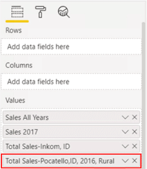
Illustration 24: Total Sales-Pocatello,ID, 2016, Rural Added to Values in the Fields Tab
Our most recent addition joins the matrix, as depicted. The value of the Total Sales-Pocatello,ID, 2016, Rural measure agrees with the value for the total sales filtered by year 2016; Pocatello. Idaho; and (as we can see, with the help of the ability to drill down from the City level to the Product Category, which we built into our Reference Data table earlier) products classified within the “Rural” category.
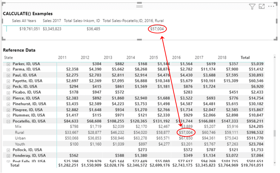
Illustration 25: Total Sales-Pocatello,ID, 2016, Rural Agrees to the Reference Data Aggregation
Let’s wrap up our basic introduction to CALCULATE() with more examples that focus upon how CALCULATE() enables us to switch context.
CALCULATE() and Context
Second Matrix Visualization
We’ll start with a fresh matrix, dedicated simply, by its design, to 2017 Sales in Pocatello, ID. We will locate the new visualization between the first CALCULATE() Example matrix, within which we have just been working, and the Reference Data matrix we’ve put in place for checking our calculations.
- Collapse the Reference Data matrix (grab and drag the top handle of the visual) enough to make room between it and the CALCULATE() Example matrix above it.
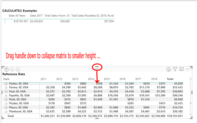
Illustration 26: : Create Space for the New Matrix by Collapsing the Reference Data Matrix
- Click the cursor on the canvas in the blank space between the CALCULATE() Examples and Reference Data matrices.
- Click the matrix icon in the collection atop the Visualizations tab, once again, to create a blank matrix on the canvas.
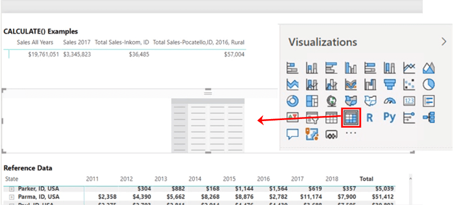
Illustration 27: Create a New Matrix between the Existing Matrices
- Drag the City column from the Geography table, in the Fields pane, to the Rows section on the Fields tab for the new visualization.
- Drag the Year column from the Date table, in the Fields pane, to the Columns section on the Fields tab for the new visualization.
Rows and Columns settings on the Fields tab appear as shown.
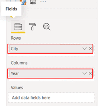
Illustration 28: Rows and Columns Settings on the Fields Tab
The new matrix visualization, at this stage, appears as depicted.
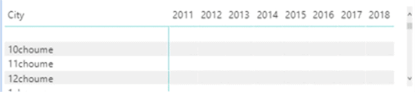
Illustration 29: Initial View of the New Matrix Visualization
- Set a visual-level filter of “City is Pocatello, ID, USA,” using the Search capability (within Basic filtering) to quickly locate the targeted filter within a long list of Idaho cities.
- Set a visual-level filter of “Year is 2017.”
Filter settings should appear as shown for the new matrix.
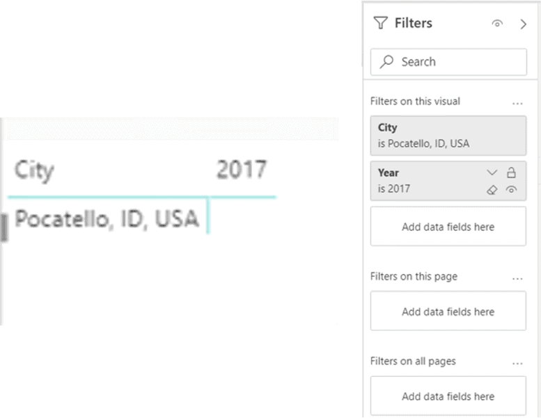
Illustration 30: Filter Settings for the New Visualization
Now that we have a context built into this matrix (via the Row and Column filters we’ve added), let’s add a few measures – a couple we’ve already created, to demonstrate the influence context has upon it what they return, and a new one to demonstrate how we can further shift context.
Example 5: Reuse a Measure Containing an Unfiltered CALCULATE() within a new Context
- Drag the Sales All Years measure we created earlier from the Sales table (Fields pane), to the Values section on the Fields tab for the new matrix visualization.
- Turn off Column Subtotals (Subtotals section) for the visualization in the Format tab (below the Visualizations collection in the Visualizations pane), as shown.
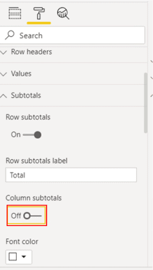
Illustration 31: Turn Off Column Subtotals …
- Also, within the Format tab, turn on Title, expand the section, and type “CALCULATE() and Context” into the Title text box, as depicted. (We can adjust the format as desired within the Title section.)
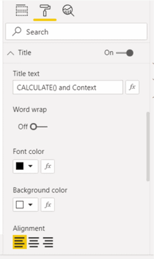
Illustration 32: Add a Title for the New Matrix
The new matrix appears as shown with the first measure added and other modifications. We can easily agree the value to be the 2017 value for Total Sales in the Reference Data matrix.
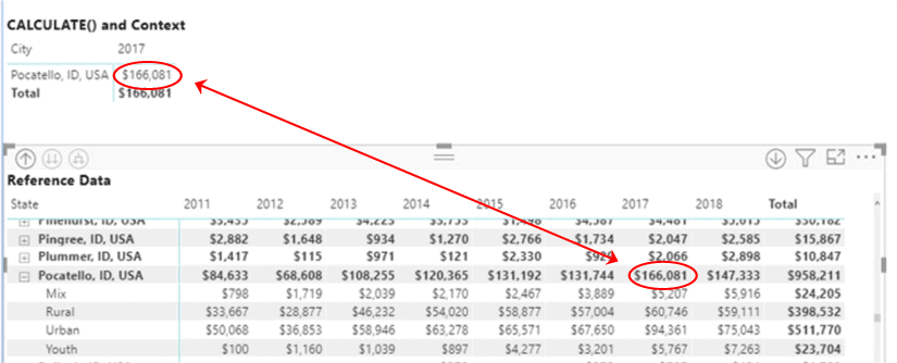
Illustration 33: Filter Settings for the New Visualization
We can easily agree the totals to be accurate for Pocatello in 2017. The calculation for the measure, we recall, is as follows:
Sales All Years = CALCULATE([Total Sales])
Nowhere within the calculation is the year filtered for 2017, so obviously the context of the measure is determined by the context of the visualization, of which the relevant focus here is year 2017 and city Pocatello, ID, USA. (We see the same calculation returning total sales for all years, all Idaho cities in the CALCULATE() Examples matrix above this one – a matrix with Idaho as the only physical filter.)
Example 6: Simple Context Transition using CALCULATE() with Filters
Let’s do another simple context transition, this time via another calculation we created earlier, Total Sales-Inkom, ID, which limits the Total Sales measure to sales in Inkom, Idaho. The calculation behind the measure, we recall, is simply:
Total Sales-Inkom, ID = CALCULATE([Total Sales], Geography[City]="Inkom, ID, USA")
- Drag the Total Sales-Inkom, ID measure we created earlier from the Sales table (Fields pane), to the Values section on the Fields tab for the new matrix visualization.
The CALCULATE() and Context matrix now appears as shown.
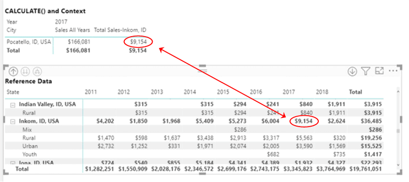
Illustration 34: Filter Settings for the New Visualization
We can again verify accuracy of the calculation via the Reference Data matrix (the value in the row Inkom, ID, USA for column 2017): the Total Sales-Inkom, ID measure we just placed in the CALCULATE() and Context matrix returns precisely what we have asked of it – regardless of the Pocatello, ID row context of the matrix itself.
NOTE: Were the title not detailed as to precisely what the value represented, the visual specification of Pocatello in the row might mislead readers with what the new calculation appears to represent. Hence the name of a measure should be precise – and should be visible – in such cases. Naming measures, always a step that requires careful planning, often becomes a challenge when we consider the many contexts – well labelled or not – within which our calculations might find themselves.
The Year stipulated in the CALCULATE() and Context matrix remains 2017 – it is not overriden within the Sales ID - Inkom measure, as year is not specified as a filter within the CALCULATE() function therein.
Example 7: Context Transition using CALCULATE() with ALL()
Now let’s create a final calculation – a calculation that overrides the single year filter (2017) enforced by the CALCULATE() and Context visualization. This time, we’ll accomplish the override via CALCULATE() in combination with another “context shifting” DAX function, ALL().
- Create a new measure called Sales All Years (ALL) within the Sales table:
Formula:
Sales All Years (ALL) = CALCULATE(SUM(Sales[Revenue]), ALL('Date'[Year]))
Format:
Currency, 0 decimal places
- Click the check mark icon on the left side of the Formula bar to commit the new measure.
Here, we are employing the ALL() function, within CALCULATE(), to reset the Date filter (per the visualization context of 2017) to “All Dates.”
NOTE: For an introduction to the DAX ALL() function, see Stairway to DAX and Power BI - Level 13: Simple Context Manipulation: Introducing the DAX All() Function.
Let’s add the new measure to our CALCULATE() and Context matrix to see context override in action.
- Select the CALCULATE() and Context matrix visualization, once again, and add the new Sales All Years (ALL) measure to the Values section of the Fields tab for the matrix (underneath the Sales ID - Inkom value we added earlier), as depicted.
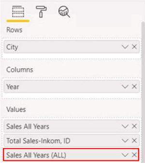
Illustration 35: Sales All Years (ALL) Added to Values in the Fields Tab
As we learned in Level 13, the DAX ALL() function is useful for clearing filters – in this case it returns all the values in the Year column of the Date table, and overrides the Year 2017 filter put into place via the matrix visual contents. I use ALL() within CALCULATE() relatively frequently within client engagements, most typically when a requirement involves a “percent of total” or “contribution to total,” etc., where we need to divide a value by the total of that value (as we see in Level 13 of this Stairway).
The context of “Pocatello, ID” remains in place for the new calculation, as nothing within the CALCULATE() function modifies it. The only mechanical / visualization filter manipulated is that of Date.Year, set to 2017 in the matrix. The ALL() function within the CALCULATE() function removes the Year filter, thus resetting the context to “All Years.” Our useful Reference Data matrix bears this out, as we can easily see.
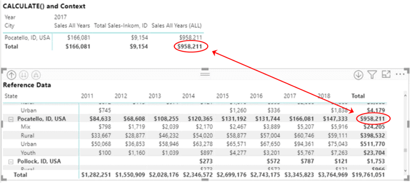
Illustration 36: Pocatello, ID Sales for All Years, Overriding the Context of the Matrix (2017)
I hope that the simple exercises we have undertaken together in this Level have helped to illustrate the operation of the DAX CALCULATE() function at its most basic – especially how it allows us to specify / shift context to meet business needs. Now that we’ve introduced its most rudimentary uses, we’ll be prepared to explore, throughout the Stairway to DAX and Power BI series, more sophisticated functional logic within the highly versatile CALCULATE() to efficiently deliver precise results from our Power BI models.
Summary
In this Level of the Stairway to DAX and Power BI series, we exposed the DAX CALCULATE() function. We discussed the general purposes and operation of CALCULATE(), and then focused upon using CALCUATE() to evaluate expressions in a context that is modified by the filters that it specifies. As part of our discussion, we examined the syntax involved with using CALCULATE(), and then constructed several basic, illustrative examples of the uses of the function in practice exercises. With each example, we explored the results datasets we obtained.
This article is part of the parent Stairway to DAX and Power BI.