In Level 17: Time Intelligence Functions: The DAX DATEADD() Function, you were introduced to the DAX Time Intelligence functions, beginning with the DATEADD() function. You learned that Time Intelligence represents a subset of the DAX formula language that supports the generation of time-specific analysis and the manipulation of data using time periods, including days, months, quarters, and years. These functions enable you to build and compare calculations over those periods.  In this Level, you will meet the DAX OPENINGBALANCEMONTH(), OPENINGBALANCEQUARTER(), and OPENINGBALANCEYEAR() functions. These functions, like other level- and interval- specific Time Intelligence functions, are “hardcoded” to support ease of selection by authors and developers, and are named for ease of selection by developers, analysts and report authors.

Operating only upon a date column, OPENINGBALANCEMONTH(), OPENINGBALANCEQUARTER(), and OPENINGBALANCEYEAR() return the opening balance for a selected month, quarter and year, respectively, within an active filter context.  As you’ll see in this Level, a typical use of the OPENINGBALANCEMONTH(), OPENINGBALANCEQUARTER(), and OPENINGBALANCEYEAR() functions is to find the corresponding occurrence of an opening balance value – even when further limiting the returned occurrence by other criteria, such as a specified location, product, or so forth.

As I’ve stated throughout this subseries, Time Intelligence functions provide a convenient means for creating calculations that provide insight into other calculations / values, and you’ll readily see how this is possible with the OPENINGBALANCEMONTH(), OPENINGBALANCEQUARTER(), and OPENINGBALANCEYEAR() functions. As is always the case with the Levels of this Stairway, the objective is to introduce each within the setting of a relatively typical business need. You will likely encounter them in the business environment, as a part of various requirements where “opening” month, quarter or year balances occurrences of a given account are a focus of a given report or another query. (In the business environment, these balances would not likely be redundantly displayed, side-by-side, with “Year-to-Date” or other values, as you assemble and display them  in this Level. The idea here is to provide corroborating values as a “self-check” mechanism.  In the business environment a given “closing balance” would likely be presented in standalone fashion.)

Illustration 1: “Opening Balance” Functions at Work

You’ll create a measure each, as you work through the various functions in this Level, that demonstrates the use of the respective function in a simple scenario, within a consolidated Matrix visualization you’ll construct.  Combining the functions within the same Matrix will allow comparison and contrast. This approach means that Time Intelligence functions can be grouped into logical Stairway Levels, and that multiple functions (four, within this case) can be explored within a single Level of the Stairway.

Additional Considerations for Time Intelligence Functions: Date Table Design Requirements

As has been the case with the other Time Intelligence functions within this Level of the Stairway to DAX and Power BI series, I will include the same reminder that I share in any Level where we work with DAX Time Intelligence functions:  It is important to remember that these functions rely upon a properly formed Date table to operate effectively.  If you are already aware of the considerations involved, you can skip to the next section.

Requirements of the Date table are as follows:

• The Date table must contain all days for each year involved.
  • Calendar Years: Each year must begin on January 1 and end on December 31.
  • Fiscal Years (only): Include all dates from the first to the last day of a fiscal year. Example: if the fiscal year 2022 starts on July 1, 2022, then the Date table must include all the days from July 1, 2022 to June 30, 2023.
• There needs to be a column (usually called Date) with a DateTime or Date data type, containing unique values.

• The Datecolumn is not required to define relationships with other tables, although it often does.
• The Datecolumn must contain unique values.
• If the Datecolumn contains a time part, the time part should not contain anything except a consistent placeholder – for example, the time would always be 12:00 AM.
• The table must be marked as a Date table in the model (via the Mark as Date Table setting), in case the relationship between the Date table and any other table is not based on the Date.
• The Datecolumn should be referenced within the enacted Mark as Date Table

NOTE:  For details regarding marking a table as the Date table, see the following: https://docs.microsoft.com/en-us/power-bi/transform-model/desktop-date-tables

Meeting the Date table requirements ensures that Time Intelligence function output complies with the data lineage of the date column or table provided as an argument.

Hands-on practice with the OPENINGBALANCEMONTH(), OPENINGBALANCEQUARTER(), and OPENINGBALANCEYEAR() functions in the next sections will make their respective objectives and operations clearer.  You’ll see, within this combined (while comparative) exploration of these functions, how each can be easily employed to return “opening” data, within the active filter context, to enable you to meet the requirements of clients or employers in the business environment. You’ll get an understanding of the purpose of each function, and gain hands-on insight into how it performs, via measures you’ll construct.

Moreover, you will:

• Examine the syntax involved in exploiting each function;
• Undertake an illustrative example of the use of each function in a practice exercise;
• Review a discussion of the results you obtain in each of the steps of the practice exercise.

Preparation for the Practice Exercises in this Level

Assuming that you have installed Power BI Desktop (the illustrations in this Stairway Level reflect the June 2023 release), you are ready to download and open the sample Power BI Desktop file that you will use for hands-on practice with the concepts introduced in this Level.

NOTE:  The latest version of the Power BI Desktop application is available for free download at www.powerbi.com.

Download Sample Power BI File (.pbix) for Use in this Level

The sample Power BI file you’ll be using contains fully imported data, and a host of pre-existing calculations and visualizations that might be helpful to you in general. Calculations created in other Levels of the Time Intelligence subseries, at least up to the time of your download, will also appear (with a “z_” prefix). You will add the calculations and visualizations that form the focus in this step-by-step Level as you go.

To complete the exercises in a given Level, I suggest that, working on a blank tab as directed throughout, you complete the steps, and then compare your results with those pre-existing in the sample.  This approach will likely produce the best learning outcome.

Using the sample dataset provided will ensure that the results you obtain in following the detailed steps of the exercises agree to the results I obtained in writing this Level, and that I have depicted in the Stairway Level, as you progress.

Once the sample .pbix file is downloaded, take the following steps to open it in Power BI Desktop.

1. Open Power BI Desktop.
2. Select Open other reports from the splash dialog that appears upon entry, as shown.

Illustration 2:  Select Open Other Reports on the Splash Dialog that Appears

3. Navigate to the file you have downloaded.

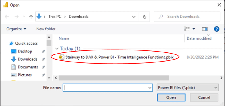
Illustration 3:  Select the Downloaded Stairway to DAX File and Open …

4. Select the file and click “Open.”

The .pbix file opens and you arrive within the Report view, which consists of several tabs (“EXERCISE EXAMPLES”) containing the solutions to the current Level, as well as solutions for past Time Intelligence subseries Levels, depending upon the date of your downloading the sample for this Level.  As you are likely aware, you can tell you are in the Report view because the current view (of the three views available in the upper left corner, Report, Data, and Model) is indicated by the colored bar to the left of the icon.

2. Click the Data and Model view icons, along the upper left frame of the Power BI Desktop canvas, as desired, to become familiar with the sample model, and then return to the Report

“Opening Balances:” The DAX OPENINGBALANCEMONTH(), OPENINGBALANCEQUARTER(), and OPENINGBALANCEYEAR() Functions

The operations, and potential uses, of the DAX OPENINGBALANCEMONTH(), OPENINGBALANCEQUARTER(), and OPENINGBALANCEYEAR() functions are very similar, except that each function contains an embedded periodicity, as indicated by its respective title. I combine the explanation of these otherwise similar functions in this section of the Level.

Discussion

Except for their names, the DAX OPENINGBALANCEMONTH(),OPENINGBALANCEQUARTER(), and OPENINGBALANCEYEAR() functions are identical in general syntax – the “behind the scenes action” embedded in the operation of each is indicated by the period suffix of its name.

Syntax

Syntactically, the parameters you provide are the same, and specified within the parentheses to the right of each function’s name, as you can see in this section:

OPENINGBALANCEMONTH()

OPENINGBALANCEMONTH(<expression>,<dates>,<filter>)

OPENINGBALANCEQUARTER()

OPENINGBALANCEQUARTER(<expression>,<dates>,<filter>)

OPENINGBALANCEYEAR()

OPENINGBALANCEYEAR(<expression>,<dates>,<filter>)

The parameters for each function are:

• Expression – The expression that returns a scalar value
• Dates – A column that contains dates
• Filter – (Optional) An expression that specifies a filter to apply to the current context.

Further Considerations

• The dates argument can be any of the following:
  • A reference to a date/time column,
  • A table expression that returns a single column of date/time values,
  • A Boolean expression that defines a single-column table of date/time values.

• A Boolean expression filter is an expression that evaluates to TRUE or FALSE. Relevant rules include the following:
• • They can reference columns from a single table.
  • They cannot reference measures.
  • They cannot use a nested CALCULATE() function.
• They cannot use functions that scan or return a table unless they are passed as arguments to aggregation functions.
• They can contain an aggregation function that returns a scalar value.
• The “Opening Balance” functions are not supported for use in DirectQuery mode when used in calculated columns or row-level security (RLS) rules.

The OPENINGYEAR() function affords a string-literal year_end_date parameter that is required for accurate operation within a fiscal year environment.  While this sort of complication is often omitted in other articles, where, perhaps, such parameters are not needed within the immediate sample(s), etc., I find that performing my articles using a fiscal year example allows practical examination of the use of the parameter, and adds utility to the Level covering the function. If you happen to be looking to implement the function in a calendar year environment, you can simply omit the year_end_date parameter.

Return Value

According to the Data Analysis Expressions (DAX) Reference, the OPENINGBALANCEMONTH(), OPENINGBALANCEQUARTER(), and OPENINGBALANCEYEAR() functions each return a scalar value that represents the expression evaluated at the first date within the specified periodicity (month, quarter, or year) context.

You’ll “meet” the “Opening Balance” functions in the Practice section that follows.  As I’ve noted, they are quite similar (with a small, additional consideration for the OPENINGBALANCEYEAR() function, as mentioned already), so introducing them this way makes it easier for you cover more in less time.

Preparation and Practice

You can easily gain an understanding of each of the OPENINGBALANCEMONTH(), OPENINGBALANCEQUARTER(), and OPENINGBALANCEYEAR() functions by putting them into action within a compact sample data set like the one in the provided Power BI model.  You will work via simple measures you create in Power BI, and be able to gain confidence that the practice measures perform correctly through viewing the results you obtain via a “self-checking” scenario. Because the three functions with which you will be working in this section are virtually identical in mechanical operation (again, with the possible exception, within your own environment, of the OPENINGBALANCEYEAR() function), you can combine your practice efforts with the group into one Matrix visual.

You’ll begin with a simple reporting requirement: to present results of each of the “Opening Balance” functions based upon some data you pull into a simple Power BI report.   Keep in mind the versatility that is possible within the Power BI application to design visualizations so that you can essentially perform “custom” queries at runtime – slicers, for example, might be added to narrow analysis to various years, various locations, and combinations of these and many other dimensional parameters.  Use your imagination to design your reports to offer multiple possible uses!

Once you have a Matrix visual in place for this purpose, you will create four new measures to demonstrate the operation of each of the DAX OPENINGBALANCEMONTH(), OPENINGBALANCEQUARTER(), and OPENINGBALANCEYEAR() functions – four because you’ll create a simple measure to support the practice exercises, and a measure to contain an example of each of the three functions. Adding these measures to the same Matrix will provide instant visual verification that the functions deliver the appropriate data (in this case values) in the manner that you expect.  The fact you’re presenting the calculation output in a Matrix visualization will allow you to generate and examine multiple outputs in a single view; it is my hope that the option to drill up / down via the Matrix will assist you as much it does me in focusing upon the action at specific levels of the data hierarchy, either together or separately.

Practice Exercises: Illustrate the Operation of the DAX “Opening” Functions through Individual Measures You Create

To prepare for some hands-on exposure to the OPENINGBALANCEMONTH(), OPENINGBALANCEQUARTER(), and OPENINGBALANCEYEAR() functions, you’ll create a simple, five-column Matrix visualization - to display Date (on the rows of the Matrix), Total Sales amount, and Sales YTD amount (which I use in the measures to follow); and then three measures, to display SalesMoOpen Bal (Opening Sales Balance for the Month), SalesQtrOpen Bal (Opening Sales Balance for the Quarter), and SalesYrOpen Bal (Opening Sales Balance for the Year).

The Matrix will be filtered to approximate the timeframe of “the full 2018 through 2020 Fiscal Years and beyond” (July 1, 2017 to June 30, 2020 and beyond) data available in the sample model. This Matrix will resemble the one partially depicted below.

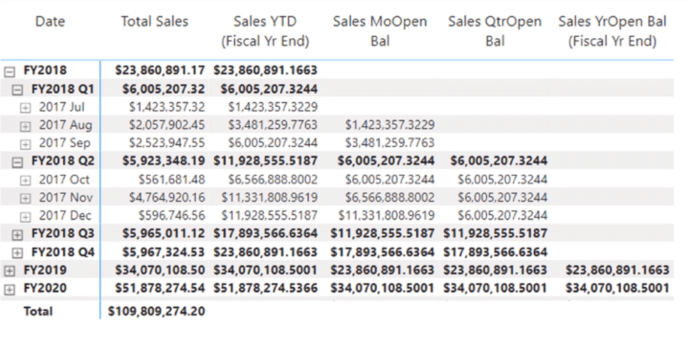
Illustration 4:  Your Goal with the Practice Matrix (Partially Collapsed View) …

NOTE: While I walk through the atomic steps of constructing the sample Matrix in the following sections, you may be new to the Power BI Matrix and want to review its general operations. Here is a good place to start for more details: https://learn.microsoft.com/en-us/power-bi/visuals/desktop-matrix-visual

Install the Matrix Visualization to Display the Date Rows

1. In the sample Power BI model, create a new tab (via the “+” button to the right of the right-most tab underneath the Power BI design area), and click-drag the tab to the Practice Canvases tabs section (to the left of the tab labelled Exercise Examples), dropping it in the location there.
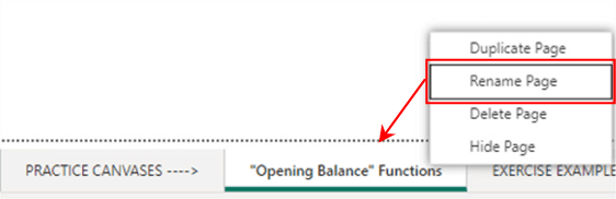
2. Right-click, and rename, the tab, as shown. (I called mine "Opening Balance" Functions, but name yours as you prefer.)

3. Click the cursor on the new tab’s blank canvas to select it.
4. Click the Matrix icon in the collection atop the Visualizations tab, to create a blank Matrix on the canvas.

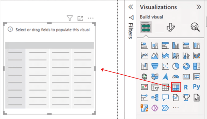
Illustration 6:  Create a New Matrix on the Canvas

5. Ensuring that the new Matrix visualization is selected, add the following table.row pairs (Data tab) to the Rows section, underneath the Visualizations collection:

• Fiscal Year
• Fiscal Quarter
• Month
• Date

Your additions should appear, within the Visualizations tab - Rows section, as shown.

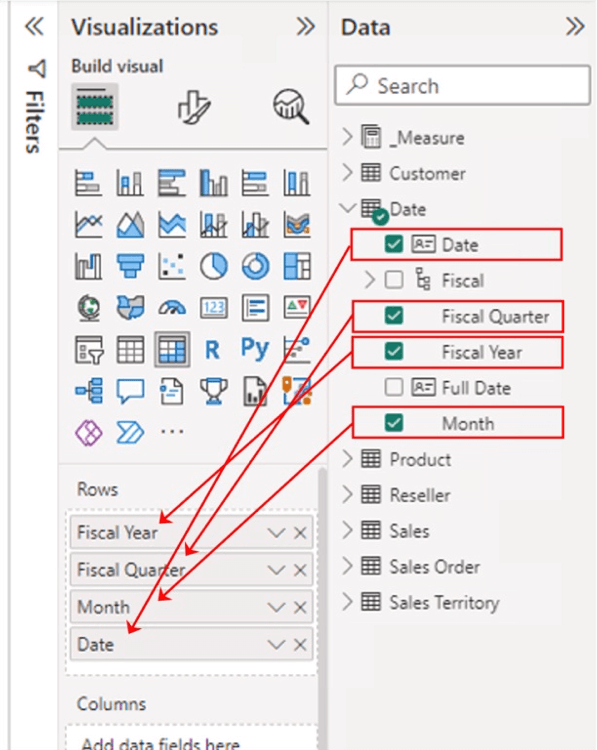
Illustration 7:  Values Additions in the Rows Section of the Visualizations Tab

While it might be accomplished at any time, you can make the top (and what will be rendered as “leftmost” in the new Matrix header) label appear as something more versatile than “Year,” as the Matrix visualization supports expanding / collapsing row headers.  It’s a good idea to keep in mind what the intended consumers of the report will see once the report is published.  Here, I will modify the label to be a more generic “Date.”  You can, of course, make it something else if you want.

6. Right-click the Fiscal Year entry in the Rows
7. Select Rename for this visual from the context menu that appears.

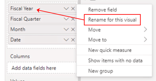
Illustration 8:  Modify the Leftmost Label in the Matrix Rows to Something More Generic …

8. Rename the row “Date,” and press the ENTER key to accept the change.

The partially expanded Matrix, at this stage, appears as depicted.

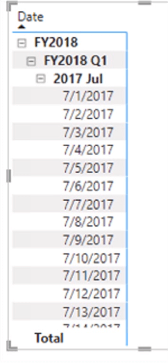
Illustration 9:  Newly Added Matrix – Partially Expanded View

Next, you will create a measure to compute Year-to-Date Sales (“Sales YTD”).  This measure will be the value upon which you generate “opening balances” values, as you’ll see in short order. Sales YTD will therefore be used throughout the exploration of the “Opening Balance” functions in this Stairway level.

Add Support Measures and Formatting to the Matrix Visualization to Get Started

1. With the Matrix on the canvas selected, add the Total Sales measure to the visualization by clicking the checkbox to the left of the measure in the Data pane, as shown.

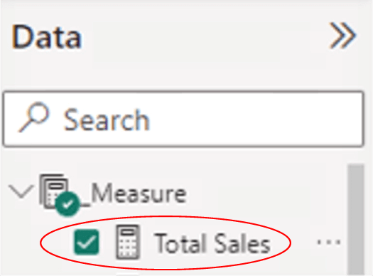
Illustration 10:  Add the Total Sales Measure to the Matrix Visualization

The new Total Sales measure is added to the Values section of the Visualizations pane, where it appears as depicted.

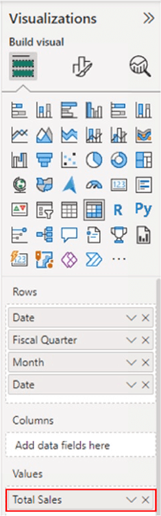
Illustration 11:  New Measure in the Values Section

The Matrix visualization appears, at this point, as partially shown (Date column assorted in ascending order, and “drilled” to the Month level).

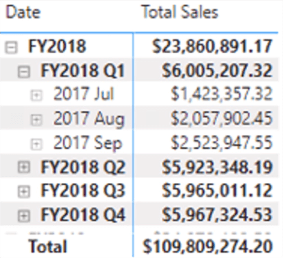
Illustration 12:  The Matrix Visualization at this Stage …

As you can see, the Total Sales measure appears to be working as expected.

Format the Matrix Visualization in Preparation for Adding the New “Opening Balance” Calculations

Having created a framework within which to work with the “Opening Balance” functions, it’s a good time to format a few points within the Matrix to enhance presentation of the data that they support.

1. With the new Matrix selected, click the Format your visual (middle) button atop the Visualizations pane, as depicted.

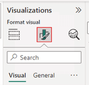
Illustration 13:  Click the Format Your Visual Button …

2. On the Visual tab of the Format pane that appears, set the following properties (and, again, you can do as you prefer):
   1. Values > Values - Font size of 12
   2. Column headers > Text – Font – Font size of 14, Header Alignment at Center
   3. Row headers > Text – Font – Font size of 12

The Values, Column headers and Row headers sections of the Visual tab appear, with modifications, as depicted:

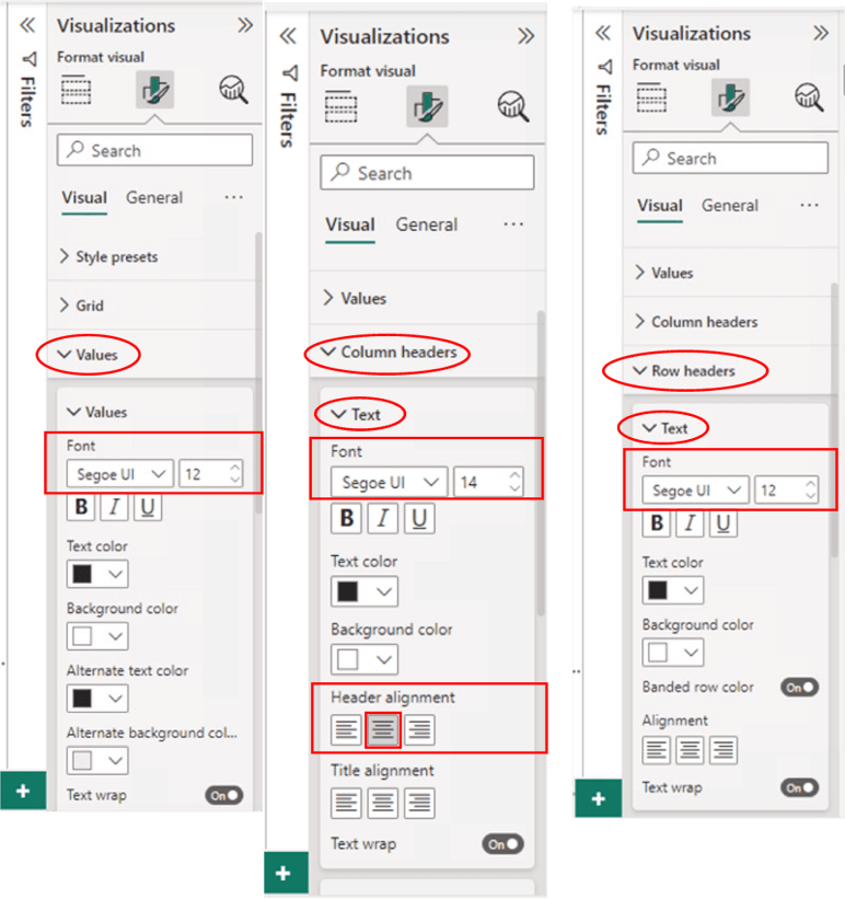
Illustration 14:  Suggested Format Adjustments (for Readability)

Create the “Year to Date Sales (Fiscal Year)” Measure - “Sales YTD(Fiscal Yr End)” - Reviewing the DAX DATESYTD() Function Covered in an Earlier Level of the Stairway

As final step in preparing to get to your work with the “Opening Balance” functions, you will create a measure to compute Year-to-Date Sales.  In Stairway to DAX and Power BI - Level 18: Time Intelligence Dates Functions, you were introduced to several assorted Dates functions, including DATESYTD(). In the example provided for using that function, you can gain an idea as to the basics for using DATESYTD() to accumulate the total of Sales to Date for a given current year, should you wish to explore the function in more detail.

Because we are working within a model with a fiscal year in this Level (and throughout the Time Intelligence functions subseries of the Stairway to DAX and Power BI), I’ll show the option for a fiscal year application with the DATESYTD() and other functions within this level.  I will only mention the difference involved in the fiscal year and calendar year operations within the affected functions as you encounter them, however, as the fiscal year option only varies in the addition of a simple string; this way, you will gain an understanding of how each affected function can be manipulated to work with either type of year.

To create the “Sales YTD (Fiscal Year End)” measure within the Matrix you’ll be using in this Level, take the following steps.

1. With the new Matrix selected, click the ellipses (“…”) to the right of the _Measure table within the Fields
2. Click New Measure atop the context menu that appears, as depicted.

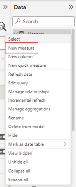
Illustration 15:  Click New Measure to Begin Design …

3. Type (or cut and paste) the following into the Formula bar for the new measure that appears:

Sales YTD (Fiscal Yr End) = 
    CALCULATE ( 
         [Total Sales], 
            DATESYTD ( 'Date'[Date], "6-30" )
)

4. Click the check mark icon on the left side of the Formula bar to commit the new measure, as shown.

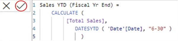
Illustration 16:  Commit the New Measure …

With this calculation, you’re creating a measure to return the “year-to-date sales” accumulation that corresponds with the current row context (as you might expect, “the date (Date column) that inhabits the row upon which the measure rests.”  While you can read more about DATESYTD() where I introduce it in Level 18 of the Stairway to DAX and Power BI, suffice it to say that this measure is being put into place to generate a “running total” for sales for the fiscal year for the respective date context selected by the user of the Matrix.

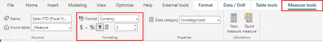
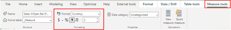
5. Ensuring that the new measure is still selected within the _Measure table, and within the Measure tools tab of the toolbar, format it as “Currency,” two (2) decimal places.

6. Add the new measure to the Matrix visualization by clicking the checkbox to the left of the measure in the Fields

The new Sales YTD (Fiscal Yr End) measure is added to the Values section of the Visualizations pane.

The Matrix visualization appears, at this point, as shown.

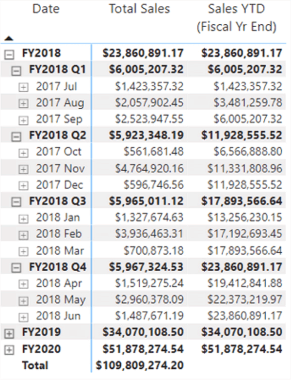
Illustration 18:  Matrix Visualization with New Measure Addition …

As you can see, the desired accumulation of the values in the Total Sales column is happening in new Sales YTD measure.

Now that we have a framework and base measure in place, it’s time to gain some exposure to the DAX “Opening Balance” functions.  To do so, you’ll create measures in the practice section that follows.

Create Measures to Support the DAX “Opening Balance” Functions

You’ll create multiple measures to demonstrate each of the OPENINGBALANCEMONTH(), OPENINGBALANCEQUARTER(), and OPENINGBALANCEYEAR() functions in action, all within an extension of the Matrix visualization you have created above. This will give you the benefit, once again, of creating “self-checking” measures within visualizations in Power BI – a convenient way to afford oneself “reasonableness” checking (and potentially more). The cumulative values delivered by measures of a given time interval (Month, for example) can be compared to the output of corresponding, higher-level (with regard to the Date dimension) measures in adjacent columns to “spot check” accuracy and completeness of the measure operation.

NOTE 1:  As I mention elsewhere within this subseries, you will see solution measures (their names are preceded by a “z_”) in the _Measure table of the Data pane. These measures are used within the EXERCISE EXAMPLES tab section to support visualization solutions in this and preceding levels of the Stairway to DAX and Power BI.  Ignore these for the time being, unless you want to use the DAX they contain, versus typing fresh the text in this Level, for copying and pasting the code into the measures that you create throughout.

NOTE 2:  You will also see, again, that there are two “title tabs” at the bottom of the downloaded Power BI model. The leftmost is labelled “PRACTICE CANVASES ---->”, and it is to the right of this tab you have been invited to place the tab(s) you create in working through the practices exercises of this Level.  To the right of the “PRACTICE CANVASES ---->” section of the tabs in the model, you will see another tab labelled “EXERCISE EXAMPLES ---->”, which borders a set of all examples we have created, to date, within the Time Intelligence subseries of the Stairway to DAX and Power BI.  The idea is to proceed in this fashion to make available a complete set of working DAX Time Intelligence examples (based upon the Level in which you are currently working) through the latest Level of this subseries.

OPENINGBALANCEMONTH() Function

Generate the Opening Sales YTD Balance for a Given Month using OPENINGBALANCEMONTH().

You’ll begin this exploration with the creation of a measure to generate a specified value as of the opening of specified month. To state this more succinctly, from an operational standpoint, what OPENINGBALANCEMONTH() actually retrieves, by design, is the closing balance from the previous month. The balance is defined by the first (expression) parameter of the function.  Moreover, the OPENINGBALANCEMONTH() function provides an optional third parameter for providing a filter.

Working with the Sales YTD (Fiscal Yr End) measure you created earlier for this purpose (remember that this is the Sales YTD computed to take into consideration a 6-30 Fiscal Year End, as explained earlier), your requirement will be to generate the opening balance for each month listed in the rows of the Matrix visualization you have assembled to this point. You can achieve this objective by taking the following steps.

1. Click the ellipses (“…”) to the right of the _Measure table within the Data
2. Click New Measure atop the context menu that appears, as you did with the measure you created earlier.
3. Type (or cut and paste) the following into the Formula bar for the new measure that appears:

   Sales MoOpen Bal = 
      OPENINGBALANCEMONTH ( 
         [Sales YTD (Fiscal Yr End)], 'Date'[Date] 
      )​
   

4. Click the check mark icon on the left side of the Formula bar to commit the new measure, again, as shown.

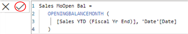
Illustration 19:  Commit the New Measure …

With this calculation, you’re creating a measure to return “the YTD Sales closing balance as of the previous month (and therefore the opening balance of the current month) relative to the current row context” (“where you are,” in this case, with regard to context in the Date hierarchy – which is dictated by the row upon which the DAX is performed).

5. Ensuring that the new measure is still selected within the _Measure table, and within the Measure tools tab of the toolbar, format it as “Currency,” two (2) decimal places.

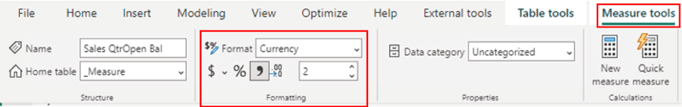
Illustration 20:  Format the New Measure …

6. Add the new measure to the Matrix visualization by clicking the checkbox to the left of the measure in the Fields

The new Sales MoOpen Bal measure is added to the Values section of the Visualizations pane.

The Matrix visualization appears, at this point, as shown.

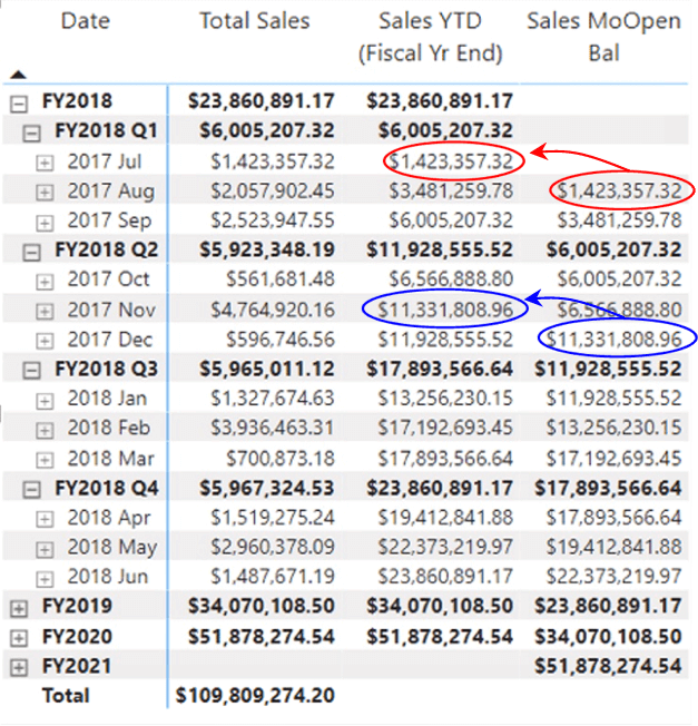
Illustration 21:  Matrix Visualization with New Measure Addition …

As you can see the Sales MoOpen Bal measure appears to be operating as expected:  The new Sales MoOpen Bal measure for each given month row (two examples are highlighted above) appears to reflect the same value as the Sales YTD (Fiscal Yr End) measure for the prior month – in effect the “ending balance” of that period as it equals the “year-to-date” value returned at that point in time.

Next, you’ll gain some exposure to the OPENINGBALANCEQUARTER() function, and create a measure to contain the function and to deliver output to the same Matrix.  Many steps will be quite similar to those you have taken with OPENINGBALANCEMONTH(), just for the quarter instead of the month.

OPENINGBALANCEQUARTER() Function

This sections shows how to generate the Opening Sales YTD Balance for a Given Quarter using OPENINGBALANCEQUARTER().

Next, you’ll create a measure to generate a specified value as of the opening of specified quarter. Another way to look at the objective, once again, might be to state, from an operational standpoint, that OPENINGBALANCEQUARTER() actually retrieves the closing balance from the previous quarter. The balance is defined by the first (expression) parameter of the function.  Moreover, as with the OPENINGBALANCEMONTH() function, OPENINGBALANCEQUARTER() supports an optional third parameter for providing a filter.

Working again with the Sales YTD (Fiscal Yr End) measure you created earlier for this purpose, your requirement will be to generate the opening balance for each quarter listed in the rows of the Matrix visualization you have assembled to this point. You can achieve this objective by taking the following steps.

1. Click the ellipses (“…”) to the right of the _Measure table within the Data
2. Click New Measure atop the context menu that appears, as you did with the measure you created earlier.
3. Type (or cut and paste) the following into the Formula bar for the new measure that appears:

Sales QtrOpen Bal = 
   OPENINGBALANCEQUARTER(
      [Sales YTD (Fiscal Yr End)], 'Date'[Date]
   )

4. Click the check mark icon on the left side of the Formula bar to commit the new measure, again, as shown.

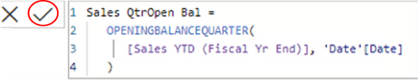
Illustration 22:  Commit the New Measure …

With this calculation, you’re creating a measure to return “the YTD Sales closing balance as of the previous quarter (and therefore the opening balance of the current quarter) relative to the current row context” (“where you are,” in this case, with regard to context in the Date hierarchy – which is dictated by the row upon which the DAX is performed).

5. Ensuring that the new measure is still selected within the _Measure table, and within the Measure tools tab of the toolbar, format it as “Currency,” two (2) decimal places.

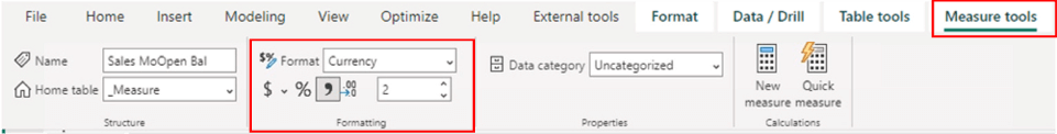
Illustration 23:  Format the New Measure …

6. Add the new measure to the Matrix visualization by clicking the checkbox to the left of the measure in the Fields

The new Sales QtrOpen Bal measure is added to the Values section of the Visualizations pane.

The Matrix visualization appears, at this point, as shown.

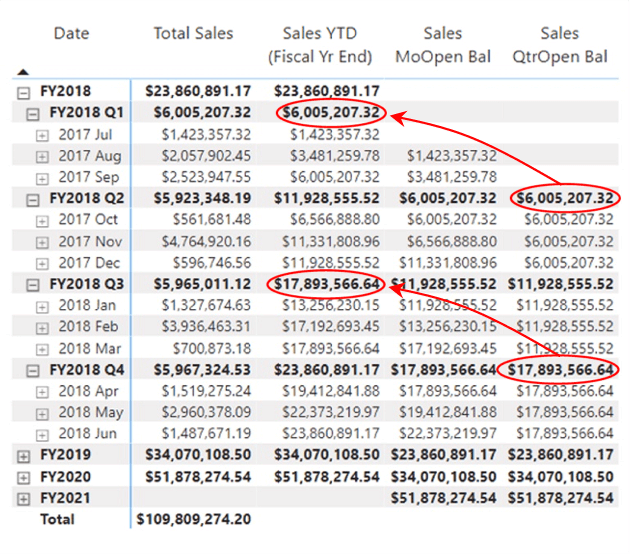
Illustration 24:  Matrix Visualization with New Measure Addition …

As you can see the Sales QtrOpen Bal measure appears to be operating as expected:  The new Sales QtrOpen Bal measure for each given quarter row (two examples are highlighted above) appears to reflect the same value as the Sales YTD (Fiscal Yr End) measure for the prior quarter – in effect the “ending balance” of that period as it equals the “year-to-date” value returned at that point in time.

Next, you’ll conclude with the OPENINGBALANCEYEAR() function, and create a measure to contain the function and to deliver output to the same Matrix.  Most steps will be quite similar to those you have taken with OPENINGBALANCEMONTH() and OPENINGBALANCEQUARTER(), just for the year instead of the quarter.

OPENINGBALANCEYEAR() Function

Next, we will generate the Opening Sales YTD Balance for a Given Year using OPENINGBALANCEYEAR(). You’ll create a measure to generate a specified value as of the opening of a specified year. Another way to look at the objective, once again, might be to state, from an operational standpoint, that OPENINGBALANCEYEAR() actually retrieves the closing balance from the previous year. The balance is defined by the first (expression) parameter of the function.  Moreover, as with the OPENINGBALANCEQUARTER() function, OPENINGBALANCEYEAR() supports an optional third parameter for providing a filter.

Working again with the Sales YTD (Fiscal Yr End) measure you created earlier for this purpose, your requirement will be to generate the opening balance for each year listed in the rows of the Matrix visualization you have assembled to this point. You can achieve this objective by taking the following steps.

1. Click the ellipses (“…”) to the right of the _Measure table within the Data
2. Click New Measure atop the context menu that appears, as you did with the measure you created earlier.
3. Type (or cut and paste) the following into the Formula bar for the new measure that appears:

Sales YrOpen Bal (Fiscal Yr End) = 
      OPENINGBALANCEYEAR(
         [Sales YTD (Fiscal Yr End)], 
      'Date'[Date], "6-30"
      )

4. Click the check mark icon on the left side of the Formula bar to commit the new measure, again, as shown.

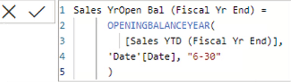
Illustration 25:  Commit the New Measure …

With this calculation, you’re creating a measure to return “the YTD Sales closing balance as of the previous year (and therefore the opening balance of the current year) relative to the current row context” (“where you are,” in this case, with regard to context in the Date hierarchy – which, again, is dictated by the row upon which the DAX is performed).

With regard to the “6-30” string literal year_end_date parameter, recall that, were we dealing with a calendar year entity here- that is, a 12-31 year end – this string could be omitted, as the logic for a 12-31 year end is built into the function. (Recall my point earlier that I have found how to use this parameter – and therefore how to handle fiscal years in specific DAX functions – overlooked in various documentation and articles, etc., I’ve come across.)

5. Ensuring that the new measure is still selected within the _Measure table, and within the Measure tools tab of the toolbar, format it as “Currency,” two (2) decimal places.

6. Add the new measure to the Matrix visualization by clicking the checkbox to the left of the measure in the Fields.

The new Sales YrOpen Bal measure is added to the Values section of the Visualizations pane. The Matrix visualization appears, at this point, as shown.

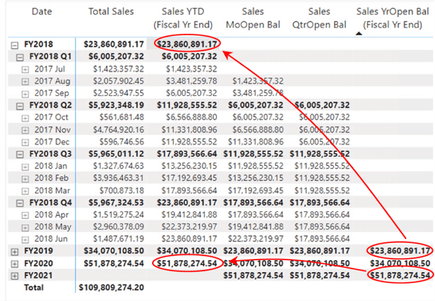
Illustration 27:  Matrix Visualization with New Measure Addition …

As you can see the new measure appears to be operating as expected:  The new Sales YrOpen Bal measure for each given year row (two examples are highlighted above) appears to reflect the same value as the Sales YTD (Fiscal Yr End) measure for the prior year – in effect the “ending balance” of that period, once again, as it equals the “year-to-date” value returned at that point in time.

You now have a set of simple Matrix visualizations that demonstrate the assembly and operation of the DAX OPENINGBALANCEMONTH(), OPENINGBALANCEQUARTER(), and OPENINGBALANCEYEAR() functions.

Summary

This Level of the Stairway to DAX and Power BI is part of a DAX Time Intelligence subseries, within which I typically introduce multiple DAX functions – grouping functions that are similar in operation in some ways, so as to condense explanations. After reading a discussion of the general purpose and operation of each of the OPENINGBALANCEMONTH(), OPENINGBALANCEQUARTER(), and OPENINGBALANCEYEAR() functions, you focused upon putting the respective function to work within the construction of a measure that demonstrated using it for reporting at summary levels similar to those you might encounter in the business environment.

As part of this introduction, you examined the syntax involved with each function, and then constructed an illustrative example of the use of the function in a simple practice exercise.  Finally, for the examples you undertook, you generated a self-validating results dataset to ensure accuracy and completeness of the results output by the measure you constructed to contain each respective function.