In Level 17: Time Intelligence Functions: The DAX DATEADD() Function, you were introduced to the DAX Time Intelligence functions, beginning with the DATEADD() function. You learned that Time Intelligence represents a subset of the DAX formula language that supports the generation of time-specific analysis and the manipulation of data using time periods, including days, months, quarters, and years. These functions enable you to build and compare calculations over those periods.  In this Level, you will meet the DAX PARALLELPERIOD() and SAMEPERIODLASTYEAR() functions.

Operating upon a date column, PARALLELPERIOD() and SAMEPERIODLASTYEAR() evaluate an expression parallel to dates in a specified column.  While PARALLELPERIOD(), as you’ll see, allows you to specify operational specifications, SAMEPERIODLASTYEAR() is significantly more limited. I cover the functions separately due to these differences, although they perform, in my opinion, similarly enough to pair in a single Level of the series.

Although the names of the PARALLELPERIOD() and SAMEPERIODLASTYEAR() functions might indicate similar output, they operate in ways that can make one more appropriate than the other, depending upon the business requirement. A summary preview of the respective actions of each might drive the reader to the section of this level that details the function that seems a better fit for the need he or she faces.

PARALLELPERIOD(), in short, works with three parameters specified: dates, a number of Intervals and an Interval. It considers the set of dates it is supplied, and, depending upon the Interval number it is given for “distance,” it looks forward or backward in time, while applying the Interval (YEAR, QUARTER or MONTH) supplied to isolate the values targeted. PARALLELPERIOD() returns full periods and not partial periods, as does another similar function, DATEADD().

NOTE 1:  For a look at my introduction to the DATEADD() function, see: Stairway to DAX and Power BI - Level 17: Time Intelligence Functions: The DAX DATEADD() Function

SAMEPERIODLASTYEAR(), in comparison, distinguishes itself from PARALLELPERIOD() upon examination – it specifies that the “parallel” or “same” period specification is “hard-wired” in its very name – as well as the Interval (a year) and the number of Intervals (negative one). SAMEPERIODLASTYEAR(), then, does exactly what its name implies, at every date level involved. Only one parameter, a date, is required.

Choosing between PARALLELPERIOD() and SAMEPERIODLASTYEAR() becomes, in effect, very simple when you consider whether you have a basic need to compare data for the same period (only) from the previous year (only), or you need / want to be able to specify a number of periods – over a single or multiple years / other Intervals (quarters or months), backward or forward in time.  PARALLELPERIOD() wins out in virtually all circumstances in my work with Power BI engagements, as PARALLELPERIOD(), by design, meets the capabilities of either function. PARALLELPERIOD() serves to be a particularly attractive option when you need a solution that lends itself to relatively simple parameterization of a given Power BI  visualization at runtime.

In next sections, I’ll detail the operation of each of the PARALLELPERIOD() and SAMEPERIODLASTYEAR() functions, providing working examples that can be recreated, and executed, in the downloadable practice .pbix file.

As I’ve stated throughout this subseries, Time Intelligence functions provide a convenient means for creating calculations that provide insight into other calculations / values, and you’ll certainly see how this is possible with the PARALLELPERIOD() and SAMEPERIODLASTYEAR() functions. As is always the case with the Levels of this Stairway, the objective is to introduce each within the setting of a relatively typical business need. You will likely encounter them in the business environment, as a part of various requirements where comparisons between periods provide a means to measure and evaluate change for various purposes.

Illustration 1: SAMEPERIODLASTYEAR() and “Parallel Periods” Functions at Work (Partially Collapsed View)

You’ll create a measure each, as you work through the various functions in this Level, that demonstrates the use of the respective function in a simple scenario, within a consolidated Matrix visualization you’ll construct.  Combining the functions within the same Matrix will allow comparison and contrast, particularly, in this case, between the two different approaches to examining periods that are adjacent in the Time dimension hierarchy.  Comparing and contrasting functions in this way has often been effective throughout the Stairway to DAX and Power BI, as it makes it possible to group “similar but also different” functions into logical Stairway Levels. In this case, two functions can be explored more efficiently, in a single Level of the Stairway.

Additional Considerations for Time Intelligence Functions: Date Table Design Requirements

At this point, I include the same reminder that I share in practically any Level where we work with DAX Time Intelligence functions:  It is important to remember that these functions rely upon a properly formed Date table to operate effectively.  If you are already aware of the considerations involved, you can skip to the next section.

The requirements of the Date table are as follows:

• The Date table must contain all days for each year involved.
  • Calendar Years: Each year must begin on January 1 and end on December 31.
  • Fiscal Years (only): Include all dates from the first to the last day of a fiscal year. Example: if the fiscal year 2022 starts on July 1, 2022, then the Date table must include all the days from July 1, 2022 to June 30, 2023.
• There needs to be a column (usually called Date) with a DateTime, or Date, data type, containing unique values.

• The Datecolumn is not required to define relationships with other tables, although it often does.
• The Datecolumn must contain unique values.
• If the Datecolumn contains a time part, the time part should not contain anything except a consistent placeholder – for example, the time would always be 12:00 AM.
• The table must be marked as a Date table in the model (via the Mark as Date Table setting), in case the relationship between the Date table and any other table is not based on the Date.
• The Datecolumn should be referenced within the enacted Mark as Date Table

NOTE:  For details regarding marking a table as the Date table, see the following: https://docs.microsoft.com/en-us/power-bi/transform-model/desktop-date-tables

Meeting the Date table requirements ensures that Time Intelligence function output complies with the data lineage of the date column or table provided as an argument.

Hands-on practice with the PARALLELPERIOD() and SAMEPERIODLASTYEAR() functions throughout the next sections will make their respective objectives and operations clearer.  You’ll see, within this combined (while comparative) exploration of these functions, how each can be easily employed to return data, within the active filter context, to enable you to meet the requirements of clients or employers in the business environment. You’ll get an understanding of the purpose of each function, and gain hands-on insight into how it performs, via measures you’ll construct.

Moreover, you will:

• Examine the syntax involved in exploiting each function;
• Undertake an illustrative example of the use of each function in a practice exercise;
• Review a discussion of the results you obtain in each of the steps of the practice exercise.

Preparation for the Practice Exercises in this Level

Assuming that you have installed Power BI Desktop (the illustrations in this Stairway Level reflect the December 2023 release), you are ready to download and open the sample Power BI Desktop file that you will use for hands-on practice with the concepts introduced in this Level.

NOTE:  The latest version of the Power BI Desktop application is available for free download at www.powerbi.com.

Download Sample Power BI File (.pbix) for Use in this Level

The sample Power BI file you’ll be using contains fully imported data, and a host of pre-existing calculations and visualizations that might be helpful to you in general. Calculations created in other Levels of the Time Intelligence subseries, at least up to the time of your download, will also appear (with a “z_” prefix). You will add the calculations and visualizations that form the focus in this step-by-step Level as you go.

To complete the exercises in a given Level, I suggest that, working on a blank tab as directed throughout, you complete the steps, and then compare your results with those pre-existing in the sample.  This approach will likely produce the best learning outcome.

Using the sample dataset provided will ensure that the results you obtain, in following the detailed steps of the exercises, agree to the results I obtained (and which I have depicted) in writing this Stairway Level.

Once the sample .pbix file is downloaded, take the following steps to open it in Power BI Desktop.

1. Open Power BI Desktop.
2. Select Open other reports from the splash dialog that appears upon entry, as shown.

Illustration 2:  Select Open Other Reports on the Splash Dialog that Appears

3. Navigate to the file you have downloaded.

Illustration 3:  Select the Downloaded Stairway to DAX File and Open …

4. Select the file and click “Open.” The .pbix file opens and you arrive within the Report view, which consists of several tabs (“EXERCISE EXAMPLES”) containing the solutions to the current Level, as well as solutions for past Time Intelligence subseries Levels, depending upon the date of your downloading the sample for this Level.  As you are likely aware, you can tell you are in the Report view because the current view (of the three views available in the upper left corner, Report, Table, and Model) is indicated by the colored bar to the left of the icon.

5. Click the Table and Model view icons, along the upper left frame of the Power BI Desktop canvas, as desired, to become familiar with the sample model, and then return to the Report

The DAX “Parallel Period” and “Same Period Last Year” Functions

The operations, and potential uses, of the DAX PARALLELPERIOD() and SAMEPERIODLASTYEAR() functions behave similarly only in cases where PARALLELPERIOD() is being used to pull a prior year balance – in short, when it is employed to behave as would SAMEPERIODLASTYEAR(). The code below illustrates an example in which both functions might be used for a similar result.

ParallelPeriod Year =
   CALCULATE([Total Sales],PARALLELPERIOD('Date'[Date], -1, YEAR)
SamePeriodLastYear =
   CALCULATE([Total Sales], SAMEPERIODLASTYEAR('Date'[Date]))

In its own respective way, each expression brings a value from the prior year.

Within the CALCULATE() function I am directing the more flexible PARALLELPERIOD() function to return the “parallel period” date, looking back (“-1”) one year, with the Interval, of a year (“YEAR”).

The SAMEPERIODLASTYEAR() function contains the Interval of “year” already, built into the function itself. All that is required to return the Total Sales value from the prior year is to is to place the Total Sales measure within the CALCULATE() function alongside the SAMEPERIODLASTYEAR() function, which contains and delivers the specific date requirements. CALCULATE(), then, has all it needs, a specified measure and a date, to deliver the value of the measure at the derived date in the past. With SAMEPERIODLASTYEAR() then, it’s easy to see that only a prior year value can be generated, as there is no option for directing that a future Date be generated.

We will craft these expressions, among others, in the upcoming exercises.  My initial objective is to illustrate how the PARALLELPERIOD() function works to deliver outputs for differing levels of the Date dimension, as well as through other criteria.  I’ll compare and contrast, at that point in our examination, the PARALLELPERIOD() function being used to work at the Year level of the Date hierarchy with a scenario where we deliver identical results, via the SAMEPERIODLASTYEAR() function, and to discuss how they differ in generating their output.

Discussion

As I will demonstrate, you can employ the PARALLELPERIOD() function to work at the three levels of the Date hierarchy – Year, Quarter and Month – by specifying one of these Intervals within the parentheses of the function, as you will see below.

SAMEPERIODLASTYEAR() works at the year level, with a “built-in” Interval. There are other assumptions built into SAMEPERIODLASTYEAR() that I discuss below. I discuss the syntax and further considerations for the PARALLELPERIOD() and SAMEPERIODLASTYEAR() functions individually in the respective sections that follow.

Function Specifics

Distinguishing characteristics between the PARALLELPERIOD() and SAMEPERIODLASTYEAR() functions appear in the following sections.

Syntax - PARALLELPERIOD()

Syntactically, the PARALLELPERIOD() function requires the same parameters regardless of whether you are specifying data at the Year, Quarter or Month Intervals. The general layout of the function is this:

PARALLELPERIOD(<dates>,<number_of_intervals>,<interval>)

The following examples illustrate the straightforward specification of each of the Intervals:

PARALLELPERIOD() for a Year

PARALLELPERIOD(<dates>,<number_of_intervals>,YEAR)

PARALLELPERIOD() for a Quarter

PARALLELPERIOD(<dates>,<number_of_intervals>,QUARTER)

PARALLELPERIOD() for a Month

PARALLELPERIOD(<dates>,<number_of_intervals>,MONTH)

The primary parameters for each function in the sequence

PARALLELPERIOD(<dates>,<number_of_intervals>,<interval>)

are as follows:

• dates – Column containing dates
• number_of_intervals – Integer specifying number of Intervals to add to, or subtract from. the dates (via no sign or a negative sign, respectively)
• interval – The Interval by which to shift dates (year, quarter, or month)

Further Considerations - PARALLELPERIOD()

• This function is not supported for use in DirectQuery mode when used in calculated columns or row-level security (RLS) rules.
• The dates argument can be any of the following:
  • A reference to a date/time column
  • A table expression that returns a single column of date/time values
  • A Boolean expression that defines a single-column table of date/time values
• If the number specified for number_of_intervalsis positive, the dates in dates are moved forward in time; if the number is negative, the dates in dates are shifted backward in time.
• This function takes the current set of dates in the column specified by dates, shifts the first date and the last date the specified number of Intervals, and then returns all contiguous dates between the two shifted dates. If the Interval is a partial range of month, quarter, or year then any partial months in the result are also filled out to complete the entire Interval.
• A Boolean expression filter is an expression that evaluates to TRUE or FALSE. Relevant rules include the following:

• • They can reference columns from a single table.
  • They cannot reference measures.
  • They cannot use a nested CALCULATE() function.
  • They cannot use functions that scan or return a table unless they are passed as arguments to aggregation functions.
  • They can contain an aggregation function that returns a scalar value.

• If the number specified for number_of_intervalsis positive, the dates in dates are moved forward in time; if the number is negative, the dates in dates are shifted backward2 in time.
• The result table includes only dates that appear in the values of the underlying table column.
• The PARALLELPERIOD() function is similar to the DATEADD() function except that PARALLELPERIOD() always returns full periods at the given granularity level instead of the partial periods that DATEADD()

As an example, if your selection of dates starts at June 10 and finishes at June 21 of the same year, and you want to shift that selection forward by one month then the PARALLELPERIOD() function will return all dates from the next month (July 1 to July 31); however, if DATEADD() is used instead, then the result will include only dates from July 10 to July 21.

NOTE 2:  For a look at my introduction to the DATEADD() function, see: Stairway to DAX and Power BI - Level 17: Time Intelligence Functions: The DAX DATEADD() Function

Syntax - SAMEPERIODLASTYEAR()

As I have mentioned, SAMEPERIODLASTYEAR(), like PARALLELPERIOD() function, returns a single column table of dates values. SAMEPERIODLASTYEAR() returns a single column table of dates values as it is “hardwired” with the year Interval, whereas the PARALLELPERIOD() function is designed to accept the quarter, month, and day Intervals, as well as the year Interval.

The general layout of the SAMEPERIODLASTYEAR() function is as follows:

SAMEPERIODLASTYEAR(<dates>)

with the <dates> column containing dates.

Further Considerations - SAMEPERIODLASTYEAR()

• This function is not supported for use in DirectQuery mode when used in calculated columns or row-level security (RLS) rules.
• The datesargument can be any of the following:
  • A reference to a date/time column
  • A table expression that returns a single column of date/time values
  • A Boolean expression that defines a single-column table of date/time values
• A Boolean expression filter is an expression that evaluates to TRUE or FALSE. Relevant rules include the following:

• • They can reference columns from a single table.
  • They cannot reference measures.
  • They cannot use a nested CALCULATE() function.
  • They cannot use functions that scan or return a table unless they are passed as arguments to aggregation functions.
  • They can contain an aggregation function that returns a scalar value.

• The dates returned are the same as the dates returned by this equivalent formula: DATEADD(dates, -1, year).

 Return Value

According to the Data Analysis Expressions (DAX) Reference, the SAMEPERIODLASTYEAR() function returns a single-column table of date values.

You’ll “meet” the SAMEPERIODLASTYEAR() function, along with the PARALLELPERIOD() function, in the Practice section that follows.  As I’ve noted, while both evaluate an expression parallel to dates in a specified column, they only produce identical results in very limited instances when they happen to be returning data within the significant limitations of SAMEPERIODLASTYEAR(). You can determine, at the time of selection and deployment, if the limited capabilities of the former will meet the needs of the business environment in which you are working, once you see the functions in action.

Preparation and Practice

You can easily gain an understanding of each of the SAMEPERIODLASTYEAR() and PARALLELPERIOD() functions by putting them into action, as we do throughout most of this Stairway, within the compact sample data set I have provided within the downloadable Power BI model.

You will work via simple measures you create in Power BI, and be able to gain confidence that the practice measures perform correctly through viewing the results you obtain via a “self-checking” scenario. Because the four functions with which you will be working in this section are quite similar with regard to output (that is, each delivers a total value relative to a point in time), you can combine your practice efforts with the group into one Matrix visual, as you will see.

You’ll begin with a simple reporting requirement: to present results of each of the four functions I have discussed above, based upon data you pull into a simple Power BI report.   The results will depict the value of the Total Sales measure, juxtaposed against the (drillable) levels of the Date dimension in the row axis of the Matrix with which we will be working in Power BI.   In this, as in many practice exercises you build within my Stairway to DAX and Power BI  series, keep in mind the significant versatility that is possible within the Power BI application to design visualizations so that you can essentially perform “custom” queries at runtime – slicers, for example, might be added to narrow analysis to various years, various locations, and combinations of these and many other dimensional parameters.  You are limited only by your imagination (and that of clients / customers to whom you offer ideas and options) in designing your reports to offer multiple possible uses!

Once you have a Matrix visual in place for this purpose, you will create four new measures: one to demonstrate the operation of the DAX SAMEPERIODLASTYEAR() function, and then three more to exhibit each of the three PARALLELPERIOD() function variants. Adding these measures to the same Matrix will provide instant visual verification that the functions deliver the appropriate data values in the manner that you expect.  The fact you’re presenting the calculation output in a Matrix visualization will allow you to generate and examine multiple outputs in a single view. It is my hope that the option to drill up / down via the Matrix will assist you, as much it does me, in focusing upon the action at specific levels of the data hierarchy, either together or separately.

Practice Exercises: Illustrate the Operation of the DAX “Same Period Last Year” and “Parallel Period” Functions

To prepare for some hands-on exposure to the SAMEPERIODLASTYEAR() and PARALLELPERIOD() functions, you’ll create a simple, six-column Matrix visualization. This will allow you to display the Date hierarchy (on the rows of the Matrix), Total Sales amount, and then a measure to display SamePeriodLastYear (the value of the Total Sales measure in the year before the one named in the Rows axis of the Matrix). Next, you’ll add the three ParallelPeriod options (the value of the Total Sales measure for Total Sales in the respective hierarchical Date level – year, quarter, or month) parallel to the one named in the Rows axis of the Matrix).

The Matrix will be filtered to approximate the timeframe of “the full 2018 through 2020 Calendar Years” (between July 1, 2017 to June 30, 2021) data available in the sample model provided with this Level. This Matrix will resemble the one partially depicted below.

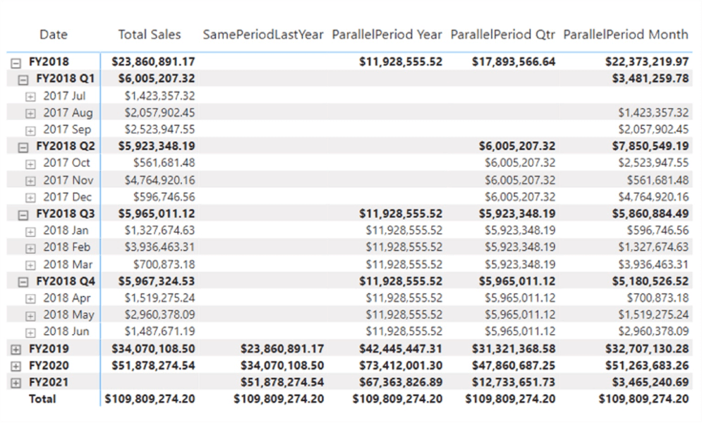
Illustration 4:  Your Goal with the Practice Matrix (Partially Collapsed View) …

NOTE: You may be new to the Power BI Matrix, and want to review its general operations, in connection with my walk through of the atomic steps of constructing the sample Matrix in the following sections. Here is a good place to start for more details: https://learn.microsoft.com/en-us/power-bi/visuals/desktop-matrix-visual

Install the Matrix Visualization to Display the Date Rows

1. In the sample Power BI model, create a new tab (via the “+” button to the right of the right-most tab underneath the Power BI design area – its default name will be “Page 1.”), and click-drag the tab to the Practice Canvases tabs section (to the left of the tab labelled Exercise Examples), dropping it in the location there.
2. Right-click, and rename, the tab, as shown. (I called mine "PARALLELPERIOD and SAMEPERIODLASTYEAR Functions,” but name yours as you prefer.)

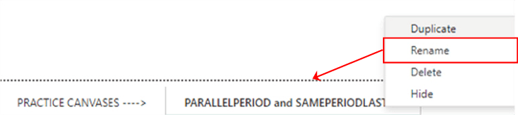
Illustration 5:  Renaming the New Practice Tab …

3. Click the cursor on the new tab’s blank canvas to select it.
4. Click the Matrix icon in the collection atop the Visualizations tab, to create a blank Matrix on the canvas.

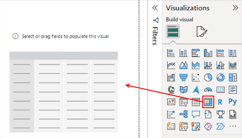
Illustration 6:  Create a New Matrix on the Canvas

5. Ensuring that the new Matrix visualization is selected, drag the following table.row pairs (Data tab) to the Rows section, underneath the Visualizations collection:

• Calendar Year
• Calendar Quarter
• Month
• Date

Your additions should appear, within the Visualizations tab - Rows section, as shown.

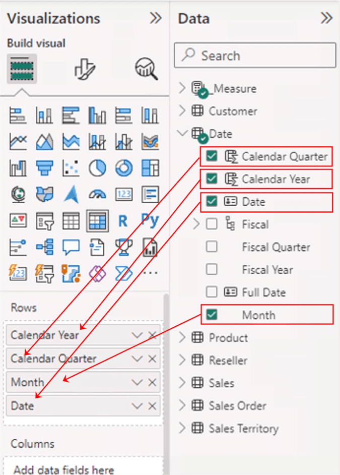
Illustration 7:  Values Additions in the Rows Section of the Visualizations Tab

While it might be accomplished at any time, you can make the top (and what will be rendered as “leftmost” in the new Matrix header) label appear as something more versatile than “Year,” as the Matrix visualization supports expanding / collapsing row headers.  It’s a good idea to keep in mind what the intended consumers of the report will see once the report is published.  Here, I will modify the label to be a more generic “Date.”  You can, of course, make it something else if you want.

6. Right-click the Calendar Year entry in the Rows
7. Select Rename for this visual from the context menu that appears.

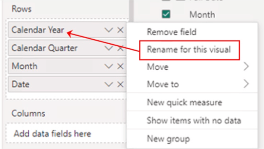
Illustration 8:  Modify the Leftmost Label in the Matrix Rows to Something More Generic …

8. Rename the row “Date,” and press the ENTER key to accept the change. The partially expanded Matrix, at this stage, appears as depicted.

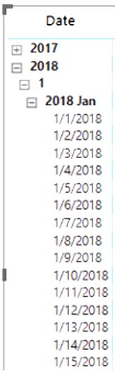
Illustration 9:  Newly Added Matrix – Partially Expanded View

Next, you will add a support measure and format the matrix a bit for a little more visual appeal.

Add Support Measures and Formatting to the Matrix Visualization to Get Started

1. With the Matrix on the canvas selected, add the Total Sales measure to the visualization by clicking the checkbox to the left of the measure in the Data pane, as shown.

Illustration 10:  Add the Total Sales Measure to the Matrix Visualization

The new Total Sales measure is added to the Values section of the Visualizations pane, where it appears as depicted.

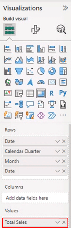
Illustration 11:  Total Sales Measure in the Values Section

The Matrix visualization appears, at this point, as partially shown (Date column sorted in ascending order, and “drilled” to the Month level).

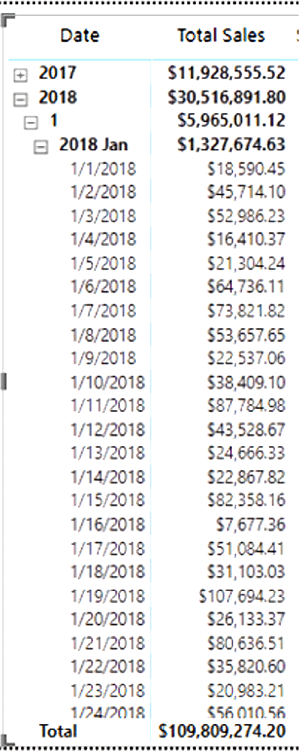
Illustration 12:  The Matrix Visualization at this Stage …

As you can see, the Total Sales measure appears to be working as expected.

Format the Matrix Visualization to Prepare for Demonstrating the Use of the Functions

Having created a framework within which to work with the SAMEPERIODLASTYEAR() and PARALLELPERIOD() functions, it’s a good time to format a few points within the Matrix to enhance presentation of the data that the functions generate.

1. With the new Matrix selected, click the Format your visual (middle) button atop the Visualizations pane, as depicted.

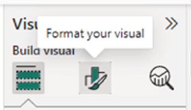
Illustration 13:  Click the Format Your Visual Button …

2. On the Visual tab of the Format pane that appears, set the following properties (and, again, you can do as you prefer):
   1. Values > Values - Font size of 12
   2. Column headers > Text – Font – Font size of 14, Header Alignment at Center
   3. Row headers > Text – Font – Font size of 12

The Values, Column headers and Row headers sections of the Visual tab appear, with modifications, as depicted:

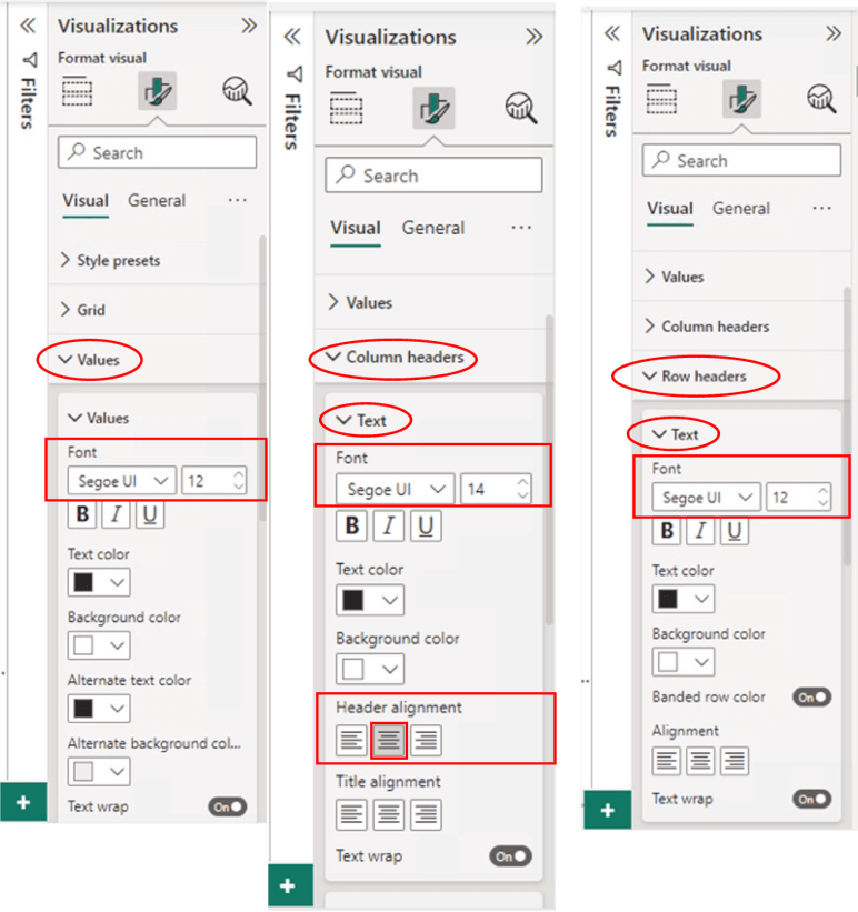
Illustration 14:  Suggested Format Adjustments (for Enhanced Readability)

Now that you have a framework and base measure in place, it’s time to gain some exposure to the DAX SAMEPERIODLASTYEAR() and PARALLELPERIOD() functions.  To do this, you’ll create measures in the practice section that follows.

Create Measures to Support the DAX SAMEPERIODLASTYEAR() and PARALLELPERIOD()  Functions

You’ll create multiple measures, one called SAMEPERIODLASTYEAR, and then three more, named ParallelPeriod Year, ParallelPeriod Qtr, and ParallelPeriod Month - these to demonstrate the use of the PARALLELPERIOD() function for each of its optional time variations.  As you’ve done in earlier Levels of the Stairway to DAX and Power BI (Time Intelligence subseries), you will create these measures within the Matrix visualization you have created above. This will give you the benefit, once again, of creating “self-checking” measures within visualizations in Power BI – a convenient way to afford oneself “reasonableness” checking (and potentially more). The cumulative values delivered by measures of a given time Interval (Month, for example) can be compared to the output of corresponding, higher-level (with regard to the Date dimension) measures in adjacent columns to “spot check” accuracy and completeness of the measure operation.

NOTE 1:  As I mention elsewhere within this subseries, you will see solution measures (their names are preceded by a “z_”) in the _Measure table of the Data pane. These measures are used within the EXERCISE EXAMPLES tab section to support visualization solutions for this and preceding levels of the Time Intelligence subseries of the Stairway to DAX and Power BI.  Ignore these for the time being, unless you want to use the DAX they contain, versus typing fresh the text in this Level, for copying and pasting the code into the measures that you create throughout.

NOTE 2:  You will also see, again, that there are two “title tabs” at the bottom of the downloaded Power BI model. The leftmost is labelled “PRACTICE CANVASES ---->”, and it is to the right of this tab you have been invited to place the tab(s) you create in working through the practice exercises of this Level.  To the right of the “PRACTICE CANVASES ---->” section of the tabs in the model, you will see another tab labelled “EXERCISE EXAMPLES ---->”, which borders a set of all examples we have created, to date, within the Time Intelligence subseries of Stairway to DAX and Power BI.  The idea is to proceed in this fashion to make available a complete set of working DAX Time Intelligence examples (based upon the Level in which you are currently working) through the latest Level of this subseries.

SAMEPERIODLASTYEAR() Function - For a Given Year, Generate Total Sales from the Previous Year with SAMEPERIODLASTYEAR()

You’ll begin this exploration with the creation of a measure that enables comparison of Total Sales between the current year and the previous year. As you’ll see, using the measure within the Power BI Matrix will support comparison with not only the same period in the previous year, but also across different time periods.

Working with the Total Sales measure you have added to the Matrix for this purpose, your requirement will be to generate the Total Sales for the same period in the previous year for each date listed in the rows of the Matrix visualization you have assembled to this point. You can achieve this objective by taking the following steps.

1. Click the ellipses (“…”) to the right of the _Measure table within the Data
2. Click New Measure atop the context menu that appears.
3. Type (or cut and paste) the following into the Formula bar(appearing above the canvas) for the new measure that appears:

SamePeriodLastYear = 
   CALCULATE(
      [Total Sales],
         SAMEPERIODLASTYEAR('Date'[Date])
   )

4. Click the check mark icon on the left side of the Formula bar to commit the new measure, as shown.

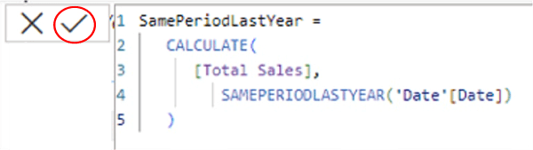
Illustration 15:  Commit the New Measure …

With this calculation, you’re creating a measure to return “the Total Sales as of the current date – in the previous year” as specified by the current row context (“where you are,” in this case, with regard to context in the Date hierarchy – which is dictated, in the Matrix, by the row upon which the DAX is performed).

5. Ensuring that the new measure is still selected within the _Measure table, and within the Measure tools tab of the toolbar, format it as “Currency,” two (2) decimal places.

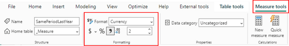
Illustration 16:  Format the New Measure …

6. Add the new measure to the Matrix visualization by clicking the checkbox to the left of the measure in the Data. The new SamePeriodLastYear measure is added to the Values section of the Visualizations pane. The Matrix visualization appears, at this point, as shown.

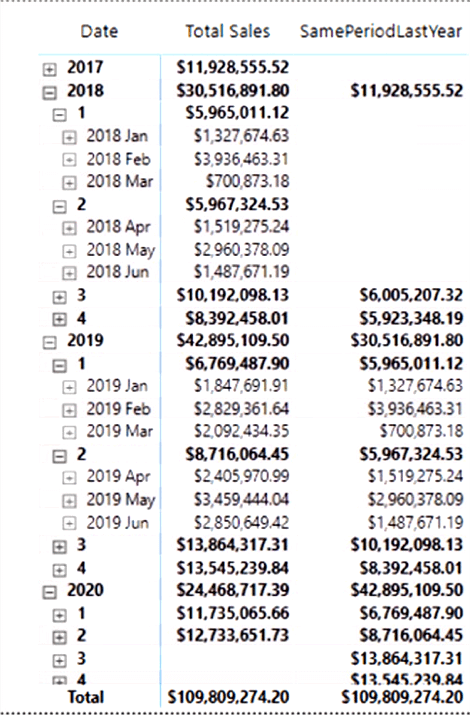
Illustration 17:  Matrix Visualization with SamePeriodLastYear Measure Addition (Partially Collapsed View)

The new SamePeriodLastYear measure appears to be operating as expected:  Its value for each given Date row appears to reflect the Total Sales value at prior-year Date levels.

Next, you’ll gain some exposure to the PARALLELPERIOD() function – in the first case working at the Year level (to facilitate side-by-side comparison with the SamePeriodLastYear measure we have already put in place). You’ll create a measure to contain the function and to deliver output to the same Matrix.

PARALLELPERIOD() Function -  For a Given Date Interval, Generate Total Sales from Previous Periods with PARALLELPERIOD()

Next, you’ll shift to an alternative way to generate values from previous periods with the PARALLELPERIOD() function. I noted earlier that that the SAMEPERIODLASTYEAR() function enables comparison of Total Sales between the current year and the previous year. While the “built in" Interval of “year” with SAMEPERIODLASTYEAR() means simplicity in its use, limitation is the price of that simplicity.

As I noted in the earlier overview, the PARALLELPERIOD() function is designed to accept the Quarter and Month Intervals, as well as the Year Interval.  Working, once again, with the Total Sales measure you have added to the Matrix for this purpose, your requirement will be to generate the Total Sales for the periods at three previous levels for each date listed in the rows of the Matrix visualization you have assembled to this point. To do so, you’ll create one measure for each of the Year, Quarter and Month Intervals. You can achieve this objective by taking the following steps, beginning with the Year Interval.

Create a Parallel Period – Year Measure

1. Click the ellipses (“…”) to the right of the _Measure table within the Data
2. Click New Measure atop the context menu that appears.
3. Type (or cut and paste) the following into the Formula bar for the new measure that appears:

ParallelPeriod Year =
CALCULATE (
    [Total Sales],
    PARALLELPERIOD (
        'Date'[Date],
        -1,
        YEAR
    )
)

4. Click the check mark icon on the left side of the Formula bar to commit the new measure, as shown.

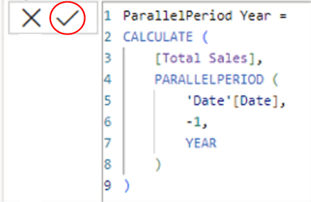
Illustration 18:  Commit the New Measure …

With this calculation, you’re creating a measure to return Total Sales as of the “parallel period of the current date” – as specified by the current row context. In the immediate example, the PARALLELPERIOD() function directs the selection of the “Total Sales value for the current date (again, determined by row context in the Matrix), looking back one (“-1”) Interval, that Interval being a year.”

In this example, we can see a couple of characteristics that make the DAX PARALLELPERIOD() function, in this case specifying a YEAR Interval, more versatile than the “hardcoded” SAMEPERIODLASTYEAR() function. First, we can specify direction, backward (-1) or forward in time - SAMEPERIODLASTYEAR() has, in effect, a “built-in” direction of “-1”. We can also specify YEAR, QUARTER or MONTH as an Interval (whereas YEAR is the preset value for SAMEPERIODLASTYEAR().  While these are key characteristics of the functions to consider in selecting a function to use in the given business environment, another consideration is the perhaps obvious advantage that the PARALLELPERIOD() function offers more variables to be parameterized, in Power BI and elsewhere, to expand runtime query capabilities (and user interaction thereby) dramatically, among other considerations. Finally, you need to keep in mind that the design of the SAMEPERIODLASTYEAR() function includes a built-in assumption that you are working with a calendar year.

5. Ensuring that the new measure is still selected within the _Measure table, and within the Measure tools tab of the toolbar, format it as “Currency,” two (2) decimal places.

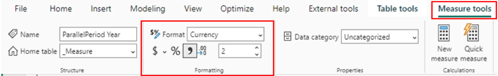
Illustration 19:  Format the New Measure …

6. Add the new measure to the Matrix visualization by clicking the checkbox to the left of the measure in the Fields

The new ParallelPeriod Year measure is added to the Values section of the Visualizations pane. The Matrix visualization appears, at this point, as shown.

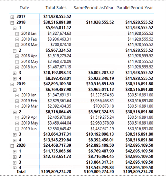
Illustration 20:  Matrix Visualization with ParallelPeriod Year Measure Addition (Partially Collapsed View)

The new ParallelPeriod Year measure appears to be operating as expected:  Its value for each given Date row reflects the Total Sales value at prior-year Date levels.

Next, you’ll gain further exposure to the PARALLELPERIOD() function – in this case working at the Quarter Interval. You’ll once again create a measure to contain the function and to deliver output to the same Matrix.

Create a Parallel Period – Quarter Measure

1. Click the ellipses (“…”) to the right of the _Measure table within the Data
2. Click New Measure atop the context menu that appears.
3. Type (or cut and paste) the following into the Formula bar for the new measure that appears:

ParallelPeriod Quarter =
CALCULATE (
    [Total Sales],
    PARALLELPERIOD (
        'Date'[Date],
        -1,
        QUARTER
    )
)

4. Click the check mark icon on the left side of the Formula bar to commit the new measure, as shown.

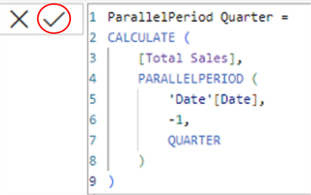
Illustration 21:  Commit the New Measure …

As you did for the Year level earlier, you’re creating a measure to return Total Sales as of the “parallel Interval of the current date” – as specified by the current row context. In the immediate example, the PARALLELPERIOD() function directs the selection of the “Total Sales value for the current date (again, determined by row context in the Matrix), looking back one (“-1”) Interval, that Interval being a quarter.”

In this case, you again demonstrate the versatility of the PARALLELPERIOD() function over the SAMEPERIODLASTYEAR() function – the primary difference being that PARALLELPERIOD() can assume an Interval other than YEAR, which is hardcoded into SAMEPERIODLASTYEAR().  Not only is  PARALLELPERIOD() more versatile than the “hardcoded” SAMEPERIODLASTYEAR() function with regard to flexible Interval selection, but you are also specifying 1) the “direction” to look forward or back in time that PARALLELPERIOD() is to take: “-1”, which is specifying “look back (‘-‘) and Interval of one quarter (‘1’).” Allowing control of the direction and the degree of look-back / look-forward is a significant expansion over the operation of the SAMEPERIODLASTYEAR() function.

5. Ensuring that the new measure is still selected within the _Measure table, and within the Measure tools tab of the toolbar, format it as “Currency,” two (2) decimal places.

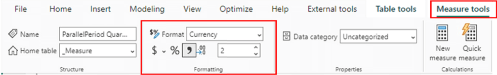
Illustration 22:  Format the New Measure …

6. Add the new measure to the Matrix visualization by clicking the checkbox to the left of the measure in the Data

The new ParallelPeriod Quarter measure is added to the Values section of the Visualizations pane. The Matrix visualization appears, at this point, as shown.

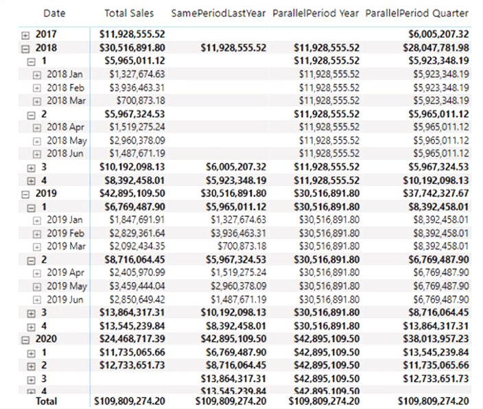
Illustration 23:  Matrix Visualization with ParallelPeriod Quarter Measure Addition (Partially Collapsed View)

The new ParallelPeriod Quarter measure appears to be operating as expected:  Its value for each given Date row reflects the Total Sales value at prior-quarter Date levels.

Next, you’ll work with PARALLELPERIOD() at its lowest Interval, Month. You’ll once again create a measure to contain the function and to deliver output to the same Matrix.

Create a Parallel Period – Month Measure

1. Click the ellipses (“…”) to the right of the _Measure table within the Data
2. Click New Measure atop the context menu that appears.
3. Type (or cut and paste) the following into the Formula bar for the new measure that appears:

ParallelPeriod Month =
CALCULATE (
    [Total Sales],
    PARALLELPERIOD (
        'Date'[Date],
        -1,
        MONTH
    )
)

4. Click the check mark icon on the left side of the Formula bar to commit the new measure, as shown.

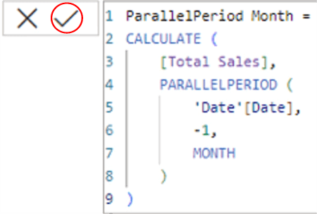
Illustration 24:  Commit the New Measure …

As you did for the Year and Quarter Intervals earlier, you’re again creating a measure to return Total Sales as of the “parallel period of the current date” – as specified by the current row context. In the immediate example, the PARALLELPERIOD() function directs the selection of the “Total Sales value for the current date (again, determined by row context in the Matrix), looking back one (“-1”) Interval, that Interval being a month.”

5. Ensuring that the new measure is still selected within the _Measure table, and within the Measure tools tab of the toolbar, format it as “Currency,” two (2) decimal places.

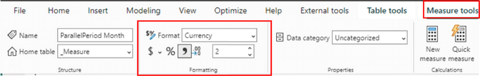
Illustration 25:  Format the New Measure …

6. Add the new measure to the Matrix visualization by clicking the checkbox to the left of the measure in the Fields

The new ParallelPeriod Month measure is added to the Values section of the Visualizations pane. The Matrix visualization appears, at this point, as shown.

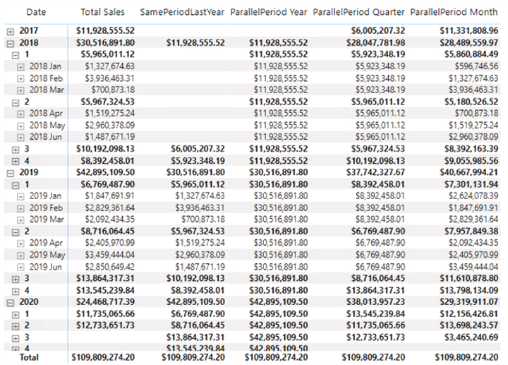
Illustration 26:  Matrix Visualization with ParallelPeriod Month Measure Addition (Partially Collapsed View)

The new ParallelPeriod Month measure appears to be operating as expected:  Its value for each given Date row reflects the Total Sales value at parallel month Intervals.

You now have a simple Matrix visualization containing measures that demonstrate the assembly and operation of the DAX PARALLELPERIOD() function in each of its possible Interval iterations.

Summary

This Level of the Stairway to DAX and Power BI is part of a DAX Time Intelligence subseries, within which I typically introduce multiple DAX functions – grouping functions, where practical, that are similar in operation in some ways, so as to condense explanations and to encourage comparison / contrast. After reading a discussion of the general purpose and operation of each of the SAMEPERIODLASTYEAR() and PARALLELPERIOD() functions, you focused upon putting the respective functions to work within a measure to meet needs similar to those you might encounter in the business environment.

As part of this introduction, you examined the syntax involved with each function, and then constructed an illustrative example of the use of the function in a simple practice exercise.  Finally, with the examples you undertook, you generated a self-validating results dataset to ensure accuracy and completeness of the results output by the measure you constructed to contain each respective function.