Introduction

In this article, I'll explain the use of the RANKX function available in DAX. The RANKX is a sortation function which is capable of performing a quite complex sorting and ranking based on the groups and values available in the dataset. It returns the ranking of a particular number available in each row of a table that forms a part of a list of numbers.

Let us first understand the basic syntax of this function.

RANKX(<Table>, <Expression>, <Value>, <Order>, <Ties>)

• Table - This is a mandatory parameter. We need to provide a table in Power BI which can either be a standard table that is imported into Power BI or a calculated table created through a DAX function. The RANKX function iterates through this table to rank a specific number in one of the columns in the table. For example, if we have a column with 10 records with values starting from 1 through 10, then the RANKX function will have the smallest possible value as 1 and the highest possible value as 10.
• Expression - This is also a required parameter. Any DAX function that returns a scalar value can be used for this parameter. The expression will iterate through each and every record in the table and return the values to be able to rank them accordingly. This can either be a simple function like SUM or some other complex functions as well.
• Value - This is an optional parameter. This is also an expression that can be evaluated in the current context. If this parameter is not provided, then the value for Expression will be used as default.
• Order - This is also an optional parameter. It specifies the order in which the rank will be applied. We can provide two values for this - 1/ASC (Ascending) and 0/DESC (Descending). This order is based on the Expression parameter. The default for this is 0; i.e. descending.
• Ties - This parameter comes into the picture in the event of a tie. It accepts two parameters - SKIP and DENSE. SKIP is used to skip the rank values in case of a tie whereas the DENSE assigns an exact count for each tie in the column. It is an optional parameter with a default value for SKIP. We will learn more about this parameter later in this article.

Solution

Now that we have some idea about how to use the RANKX function in DAX, let's go ahead and see some practical examples and uses of this function in Power BI.

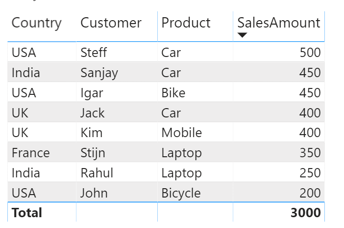
Let us also create a simple dataset with some dummy data and load it into Power BI. For this example, I've created the dataset with four columns as follows. You can download the Power BI sample along with the dataset here.

Basic Example

Let's get started with the simple implementation of the RANKX function in Power BI and generate the rank of the SalesAmount column. We will create a calculated column with the following formula.

RANKX (SalesAmount) = RANKX(Sales,Sales[SalesAmount])

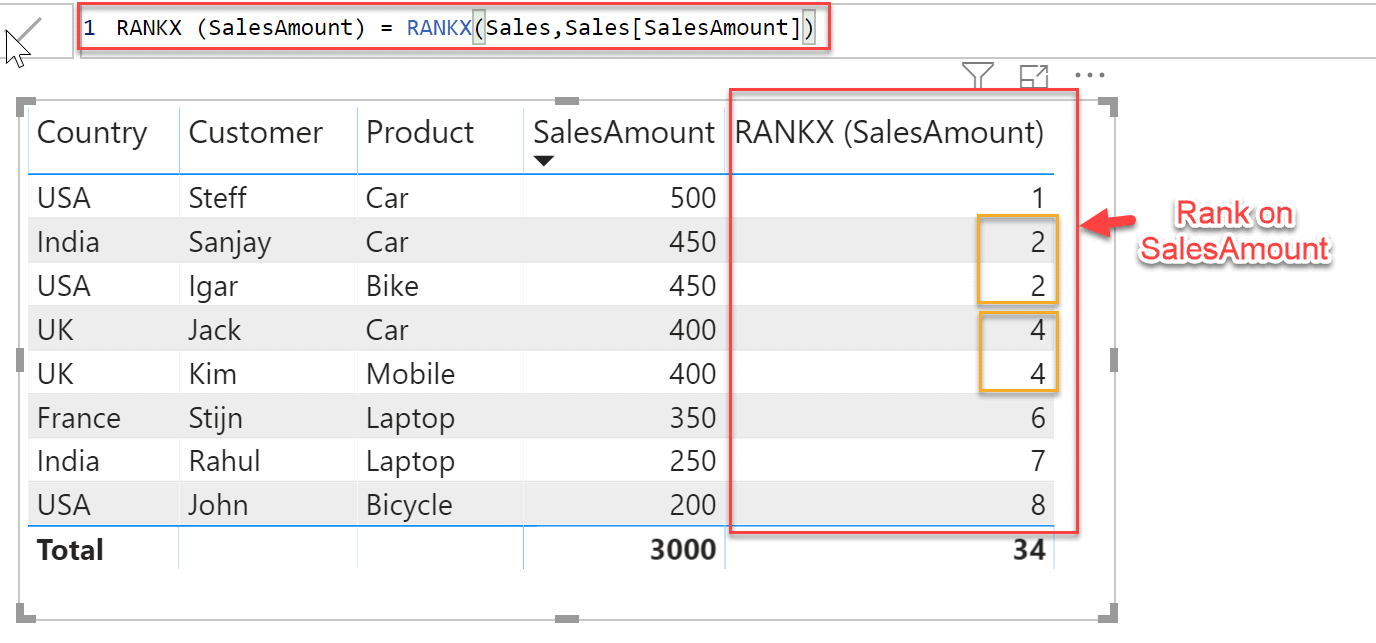
If you see the results in Fig 2, the new column RANKX (SalesAmount) has ranked the SalesAmount from the largest to the smallest value, where the largest value has a rank of 1. Also, another important thing to notice here are the ties with the ranks 2 and 4. It can be seen that for Sanjay and Igar, each has a SalesAmount of 450 has been ranked as 2, and for Jack and Kim, each having SalesAmount of 400 has a rank of 4. Thus, the rank values 3 and 5 are skipped and not included in this column.

RANKX with DENSE parameter

Now, let's create another calculated column and pass the DENSE parameter and confirm the behavior of not skipping the rank values for ties.

Dense RANKX = RANKX(Sales,Sales[SalesAmount],,,Dense)

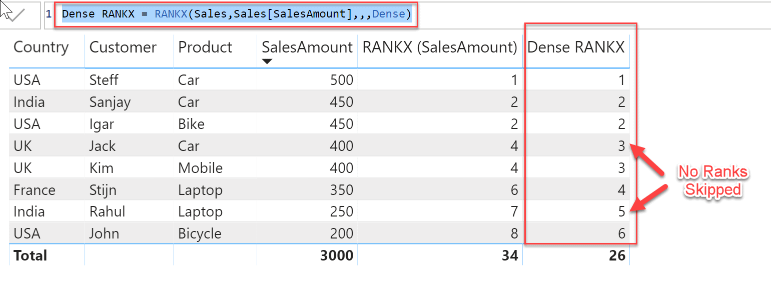
In Fig 3, it is important to note that now there are no ranks skipped in the new column Dense RANKX in case of ties. For the customers Jack and Kim, the Dense Rank now returns 3 as opposed to 4 in the previous example.

RANKX with the Order parameter

Let's create another calculated column RANKX Ascending and pass the Order parameter as ASC.

RANKX Ascending = RANKX(Sales,Sales[SalesAmount],,ASC)

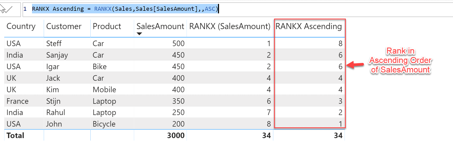
Notice in the above figure, how the rank calculation is implemented in the ascending order of the SalesAmount. The row with the lowest SalesAmount is ranked as 1 and highest as 8. Also, we have skipped the ranks 5 and 7 in this example for the ties.

RANKX with a Group

Now that we have seen some basic examples of how the RANKX function can be used to rank the rows, let's look at a more complex scenario. Suppose that you want to dynamically display the rank of SalesAmount based on a filter or some other field. In such a case, it is important to evaluate the context of the filter first and then calculate the rank based on the selected value from the filter.

In this example, let's group the rank by Country such that the rank will be calculated for each country separately.

RANKX By Group = RANKX(
    FILTER(
        Sales,
        Sales[Country] = EARLIER(Sales[Country])
    ),
    Sales[SalesAmount]
)

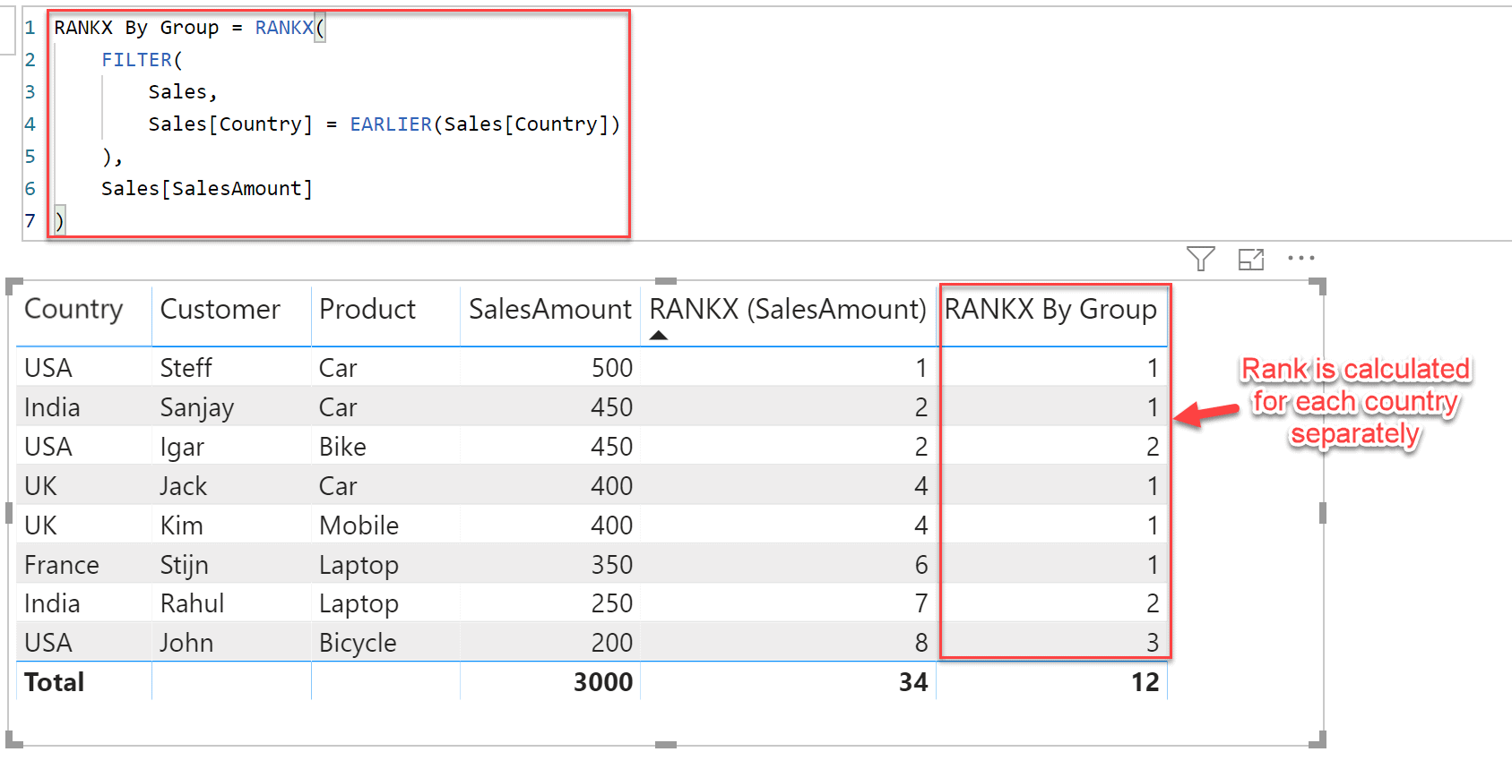
In the above figure, we can see that the rank is re-calculated for every country in the dataset. For example, let's consider the country USA. You can see that the new column RANKX By Group has rank values like 1, 2 and 3 whereas for other countries it starts with 1 again.

In the above example, we have used two other DAX functions - FILTER and EARLIER. Let's understand what these two function do in this example. The FILTER function in DAX adds an additional row context, which in essence, is a new table. So what FILTER does is it will run through every single row in our Sales table and look at what the Country name is and evaluate it based on the same value as the EARLIER Country name. What the EARLIER, does is if let’s say the USA was the first Country in our column it will iterate through the entire column and evaluate each row to see if it is the same as the first row, which is the USA. Once it iterated through the entire column it will create an additional row context against which the RANKX function will rank the values for only the USA. This iteration will then be performed for each Country and each Country’s ranking will start at 1.

Let’s take the USA as an example. Our original table has 8 rows when FILTER has iterated through the table based on the EARLIER function it will return a ‘new’ table to the RANKX function to evaluate containing only the corresponding rows based on the USA, 3 rows.

Takeaway

In this article, we have learned what is the RANKX function in DAX and how we can implement it in Power BI. We have also explored some examples and understood the logic behind the various parameters used in this function.

• For more details, you can refer to the official documentation of RANKX from Microsoft.
• See in detail about the FILTER and EARLIER functions in DAX.