Introduction

This article celebrates a classic algorithm [1] of Dijkstra (1930 – 2002) which finds a path of minimal cost between any pair of nodes in an undirected graph. His procedure is widely recognized as a fundamental tool for examining communication and transportation networks (eg. Google Maps) and is surprisingly simple. By his own admission, he solved this problem in twenty minutes while having coffee with his fiancée Ria [2].

The presentation below views his minimal path problem as coloring the nodes of a weighted undirected graph, in a certain order, to converge on a minimal path, and uses mathematical induction to ensure its optimality. It provides a simple theorem that describes the key issue, and from its proof, the algorithm follows. An overview will first explain this approach using a simple example, and then the algorithm itself is written as a by-product of that proof. Based on this, a simple SQL WHILE loop implements a solution.

Problem

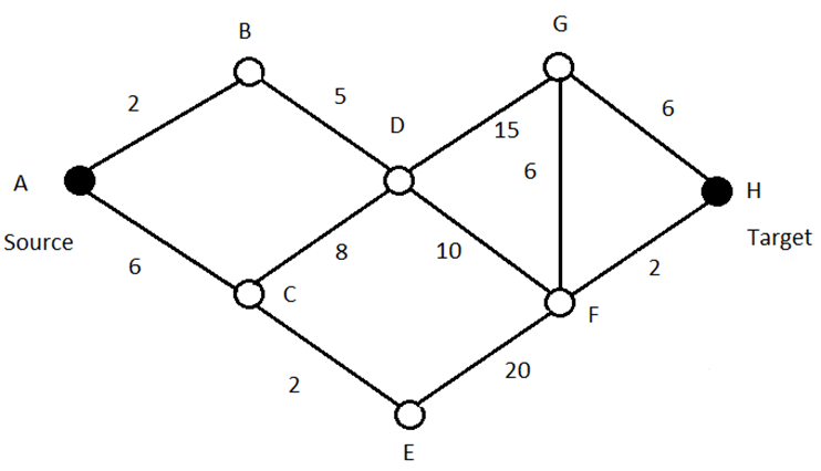
Find a path from A to H with minimal cost

Overview Of The Algorithm

Dijkstra’s algorithm is presented in the context of node coloring, with no reference to computer programming, and shows why the algorithm always works.

Node coloring, and the computations that accompany it, are a convenient way to document how to find a path to source with minimal cost from each node, one node at a time. Although this seems like overkill, these calculations are needed to derive a path from A to H with minimal cost.

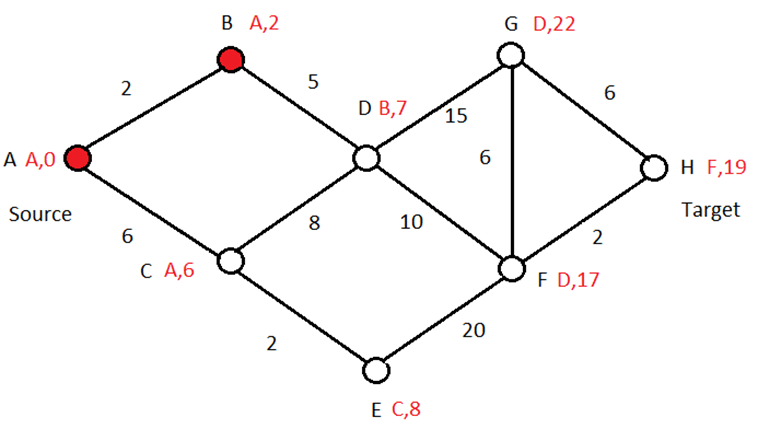
The algorithm does this by computing the red values N,C for each node, where “N,C” means “You may find a path of minimal cost C to source by first going to node N.” So, for node H, “F,19” means that a path of minimal cost 19 from H to A may be found by first going to node F. That node then says that a path of minimal cost 17 from it to source may be found by first going to node D, and so on. Continuing this way yields the path H -> F -> D -> B -> A from H to A with minimal cost 19.

That the computations below always return a path of minimal cost from A to H (or any other node) will become evident in the way they’re defined. The order in which they’re calculated is critical. After a computation is made for a given node, it will be colored red. Each such node always “knows” a minimal path for it using the nodes that have already been colored, which the remaining nodes then use to color themselves.

First, color the source red with the values A,0. Then choose a neighbor N of minimal cost C and color it red with the values A,C. So, for the above example, choose B with values A,2. Since B has minimal cost among all neighbors of A, no other path from B to A can have a lower cost since it must eventually pass through one of those neighbors. Note that to make this observation, all costs must be non-negative.

The remaining nodes will be colored in the same way, one at a time, until all “reachable” nodes are colored. When the target node is eventually colored (assuming it can be reached), its values N,C will allow us to walk back from target to source along a minimal path. When the algorithm concludes, the colored nodes will be those connected to the source by at least one path, along with instructions N,C on how to traverse a minimal path from each of them to the source. You could, of course, halt the algorithm when the target node has been colored.

The main problem is finding the next node that can be colored, along with its N,C values.

If there are no neighbors of the red nodes (A,B), then no path from A to H (or any other node) exists so the algorithm halts.

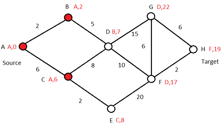
Otherwise, select one of them to color whose cost to the source node is minimal (using just the red nodes). In our example, C and D are candidates. Since the cost for C = 6 and D = 5 + 2 = 7 you may color C red with values A,6. For the same reason as before, no other path from C to A can have a lower cost. For example, C -> D -> B -> A cannot have a lower cost since the cost of D -> B can’t be smaller than the cost of C -> A, which is minimal among all neighbors. So, the cost of C -> D -> B -> A can’t be smaller than the cost of C -> A. That’s why we picked a neighbor with minimal cost to the source, using just the red nodes (whose N,C values have already been computed).

Subtle point: each neighbor may have multiple edges connecting it to the red nodes. In that case, select a red node yielding minimal cost to the source for that neighbor. So, if an edge also existed between C and B whose cost is 0, then choose that one instead (so the values of C would be B,2 instead of A,6).

Continuing this argument with the expanded set of red nodes, the remaining nodes may now be colored in the same way and in the following order: D, E, F, H, G. Note that H, for this example, is not the last node that’s colored.

Mathematical Interpretation

Call a set of nodes red if every node in that set has at least one path to the source node using just the red nodes, and at least one of them has minimal cost compared to any other path from it to the source node using any nodes in the graph. As well, every red node has values N,C where N is the next red node on some path of minimal cost, along with the cost C of that path. There may be multiple such paths of minimal cost but only one value of N is arbitrarily selected.

Clearly the source node S (with values S,0) must belong to the set. In fact, the set {S} itself may be viewed as a set of red nodes (where S has values S,0).

The neighbors of the red nodes are, by definition, those non-red nodes in the graph with at least one edge connected to a red node.

Suppose we could always add a new node to any set of red nodes, whenever that set has at least one neighbor. Then this process could continue from {S} until the latest set of red nodes has no neighbors. If the target node T has become red, we’re done. Otherwise, S and T are not connected because the latest set of red nodes has no neighbors.

Theorem

If a set of red nodes has at least one neighbor, then one of them may be added to the set

Proof

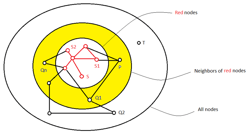
Suppose the set of red nodes has at least one neighbor. Choose a neighbor P connected to a red node S1(N1,C1) where cost(P,S1) + C1 is minimal among all its edges connected to the red nodes and for all neighbors of the red nodes. In other words, P is the “closest” neighbour to the source (and it knows how to get there). Call this value the “neighborhood minimal” of the set of red nodes, for convenience.

So, to add P to the set, it remains to show that any path from P to S using any nodes in the graph can’t have a lower cost.

Suppose P -> Q1 -> Q2 -> … is another path from P to S using any  nodes in the graph. Let Qn be the last time that path enters the set of red nodes (at S2(N2,C2), say).

Then cost(Qn,S2) + C2 can’t be less than cost(P,S1) + C1 because the latter is a neighborhood minimal.

So, cost(P,Q1) + cost(Q1,Q2) + … + cost(Qn,S2) + C2 can’t be less than cost(P,S1) + C1 since all costs are non-negative. Therefore, the new path can’t have lower cost than the original path.

You may now add P(S1,cost(P,S1) + C1) to the set of red nodes.

Algorithm

S = source node, T = target node
Set RED = {S}, Next(S) = S, Cost(S) = 0 
Set N = number of neighbors of RED
WHILE N > 0
BEGIN
Select a neighbor P of RED with neighborhood minimal value Cost(P,S1) + Cost(S1) 
for some S1 belonging to RED
Add P to RED with values Next(P) = S1, Cost(P) = Cost(P,S1) + Cost(S1) 
Set N = number of neighbors of RED
END

Upon completion, the set RED contains all nodes connected to source and for each node in RED its Next and Cost values identify the start of a minimal path to source and the cost of that path.

Script

--
-- Parameters
--
DECLARE @Graph NVARCHAR(MAX)= '
SELECT ''A'' AS Node1, ''B'' AS Node2, 2 AS Cost
UNION
SELECT ''A'' AS Node1, ''C'' AS Node2, 6 AS Cost
UNION
SELECT ''B'' AS Node1, ''D'' AS Node2, 5 AS Cost
UNION
SELECT ''C'' AS Node1, ''D'' AS Node2, 8 AS Cost
UNION
SELECT ''C'' AS Node1, ''E'' AS Node2, 2 AS Cost
UNION
SELECT ''D'' AS Node1, ''F'' AS Node2, 10 AS Cost
UNION
SELECT ''D'' AS Node1, ''G'' AS Node2, 15 AS Cost
UNION
SELECT ''G'' AS Node1, ''F'' AS Node2, 6 AS Cost
UNION
SELECT ''G'' AS Node1, ''H'' AS Node2, 6 AS Cost
UNION
SELECT ''F'' AS Node1, ''H'' AS Node2, 2 AS Cost
UNION
SELECT ''E'' AS Node1, ''F'' AS Node2, 20 AS Cost
'
DECLARE @Source VARCHAR(128) = 'A'-- You may put any node here for @Source
DECLARE @Target VARCHAR(128) = 'H'-- You may put any node here for @Target
-- Declarations
DECLARE @ROW_COUNT INT
DECLARE @Cost VARCHAR(16)
DECLARE @Path VARCHAR(MAX)
DECLARE @Node VARCHAR(128)
--  Drop table #Graph
IF OBJECT_ID(N'tempdb..#Graph') IS NOT NULL DROP TABLE #Graph
--  Create table #Graph
CREATE TABLE #Graph (
Node1 VARCHAR(128)
,Node2 VARCHAR(128)
,Cost INT 
);
-- Populate table #Graph
INSERT INTO #Graph EXEC dbo.sp_executeSQL @Graph
-- Drop table #RED
IF OBJECT_ID(N'tempdb..#RED') IS NOT NULL DROP TABLE #RED
--  Create table #RED
CREATE TABLE #RED (
[Node] VARCHAR(128)
,[Next] VARCHAR(128)
,Cost INT 
);
-- Initialize table #RED with @Source
INSERT INTO #RED SELECT @Source AS [Node], @Source AS [Next], 0 AS Cost 
-- Populate table #RED according to induction argument
SET @ROW_COUNT = -1
WHILE @ROW_COUNT <> 0
BEGIN
INSERT INTO #RED
SELECT TOP 1 d.[Node], d.[Next], d.Cost FROM-- Select top row from query
(
SELECT Graph.Node2 AS [Node], RED.[Node] AS [Next], Graph.Cost + RED.Cost AS Cost 
FROM #Graph Graph INNER JOIN #RED RED ON Graph.Node1 = RED.[Node]
WHERE Graph.Node2 NOT IN (SELECT [Node] FROM #RED)
UNION -- Required since edges have no direction
SELECT Graph.Node1 AS [Node], RED.[Node] AS [Next], Graph.Cost + RED.Cost AS Cost 
FROM #Graph Graph INNER JOIN #RED RED ON Graph.Node2 = RED.[Node]
WHERE Graph.Node1 NOT IN (SELECT [Node] FROM #RED)
) d
ORDER BY d.Cost ASC-- Pick closest neighbor to @Source
SET @ROW_COUNT = @@ROWCOUNT
END
--
-- Display answer 
--
-- Get cost of minimal path from @Target to @Source
SELECT @Cost = Cost FROM #RED WHERE [Node] = @Target  -- @Target may not belong to #RED 
IF @Cost IS NOT NULL  -- @Target belongs to #RED  
BEGIN
-- Build minimal path from @Source to @Target 
SET @Path = @Target
SET @Node = @Target
WHILE @Node <> @Source -- Loop through nodes from @Target to @Source using Next column in #RED
BEGIN
SELECT @Node = [Next] FROM #RED WHERE [Node] = @Node-- Get Next node for current node
SET @Path = @Node + ' --> ' + @Path-- Append to path
END
-- Display minimal path from @Source to @Target
SELECT @Cost AS Cost, @Path AS Path
-- Display all minimal paths
SELECT * FROM #RED
END
ELSE
SELECT -1 AS Cost, '@Source and @Path are not connected' AS Path

You may change @Source and @Target to any pair of nodes. Of course, when @Source changes so do the values of the Next column for each node in the #RED table. Also note that if both values are set to H in the above example, there are two minimal paths from E to H but the script arbitrarily selected the path of greater length because it was not concerned about how many nodes were used.

Important: Use the stored procedure sp_MinimalPath in the resource section which has performance improvements and extensive error checking on @Graph. Most processing involves populating #RED. For example, on a test machine the run-time on 8000 edges was about 3 minutes (so check the size of @Graph before proceeding). Setting @StopAtTarget = 1 will improve performance by stopping the population of #RED when @Target has been reached.

Historical Notes

In theorem-proving, an induction technique like the one above is sometimes used to prove that a finite set has a given property by first showing that any proper subset of it, with that property, can always be enlarged by adding another (carefully selected) element. So, finding any subset with that property (like {S} in our problem) would demonstrate that the complete set has that property. This won’t work for infinite sets, of course, but similar constructions may be used to prove the opposite case.

For example, Euclid showed that there are infinitely many primes by assuming that the set of all primes is finite. But by adding 1 to their product yields a larger number which won’t be in that set. And by construction, it can’t be divided by any member of that set. So, it’s either a new prime or it’s divisible by some prime that can’t be in that set. This contradicts the assumption that a finite set of all primes exists, so it must be false. Such mode of thinking, from someone who approached this problem 2,500 years ago, demonstrates the timelessness of ancient mathematical thinking and the brilliance of its thinkers.

Cantor’s famous diagonalization argument [3] is another example, where he shows that no infinite sequence of real numbers can include them all, so the set of reals is “larger” in some sense than the set of integers. This inspired a revolution in set theory, where infinite sets can now be larger than others. It was later shown [4] that it can’t be proved or disproved that some set exists that’s greater in size than the integers but smaller than the reals. So, the usual axioms of set theory need to be amended, depending on what you want to believe. This brought in the logicians who, among other things, legitimized Newton’s use of infinitesimals via Abraham Robinson’s non-standard analysis [5] and provided the foundation for Prolog [6], a well-known AI language.

Turing and Godel used similar arguments in their work about what’s computable or decidable.

Application To Human Resources

In a previous article [7] it was shown how hierarchical tables commonly used by HR may be viewed as trees when a “parent” relationship exists between records (ie. where one of its columns refers to each record’s “parent” or manager). The top node of the tree would be the company’s CEO (whose parent is NULL), all other records have a parent, and no looping occurs in the relationship. By adding and populating new columns numChildren, numDescendants, numLeaves, Height, Depth using simple CTE calculations, some complicated questions may be easily answered, such as “Which manager three steps below the CEO has the largest number of direct reports compared to all employees of that manager?.” Such questions are vital when planning corporate re-organizations.

But suppose you want to ask that question on earlier versions of the table, which no longer exist? In an upcoming article it will be shown how to convert the tree of one such table to an earlier version using an auto-generated SQL script when comparing them. Each version of the table will have its script stored (and date-stamped) in a log table. This results in a directed graph (whose direction only affects the meaning of neighbor in the above proof) whose nodes represent different versions of that tree, and whose edges connecting them represent the SQL scripts converting one node to an earlier node. By comparing today’s tree with yesterday's tree each day, the log table allows you to compare today's tree with last year’s tree, which no longer exists, by simply executing those scripts chronologically to build last year's tree from today’s. In the same way, you may add edges between any pair of trees in the past (on a weekly basis, say). Dijktra’s algorithm is then used to compute a path from today’s tree to last year’s tree involving a minimal number of SQL statements.

Resource Section

The resource section contains the above script, along with the stored procedure sp_MinimalPath and a print-ready copy of this article.

References 

[1] https://en.wikipedia.org/wiki/Dijkstra%27s_algorithm
[2] https://www.cwi.nl/en/about/history/e-w-dijkstra-brilliant-colourful-and-opinionated/
[3] https://en.wikipedia.org/wiki/Cantor%27s_diagonal_argument
[4] https://en.wikipedia.org/wiki/Continuum_hypothesis
[5] https://en.wikipedia.org/wiki/Nonstandard_analysis
[6] https://en.wikipedia.org/wiki/Prolog
[7] https://www.sqlservercentral.com/articles/verifying-trees