In this Level of the series, we continue our examination of DAX functions with the CountA() and CountAX() functions. From a high level, CountA() enables us to count the number of cells in a column that are not empty, while CountAX() affords us the capability to count nonblank results when evaluating the result of an expression over a table.

As a part of our introduction, we will discuss ways in which we can employ CountA() and CountAX(). We’ll look at each function in standalone scenarios, as well as in situations where we combine it with other functions, when appropriate, to meet the business requirements of clients, employers or peers in our own environments. During our exploration of the CountA() and CountAX() functions, we will:

• Examine the syntax involved in exploiting each
• Undertake illustrative examples of the use of each function in practice exercises
• Briefly discuss the results datasets we obtain in each of the practice examples

We will examine the output we obtain using these two functions within Power BI Desktop in the practice session that follows our overview and explanation of the purpose and operation of each function. We will create calculated columns and / or measures that put CountA() and CountAX() to work in Power BI Desktop visualizations we create, to further examine and extend the behavior that we will have observed in columns created in the Data view, particularly where evaluation context is a factor. Along the way, we will contrast differences in use and behavior of the functions in columns and measures in general, suggesting criteria to consider in choosing which of these calculation types to employ to meet the business requirements we encounter.

NOTE: For an introduction to Power BI and Power BI Desktop, see “A Brief Introduction to Power BI and Power BI Desktop” in Stairway to DAX and Power BI - Level 10: Function / Iterator Function Pairs: The DAX Product() and ProductX() Functions, where we recognize the evolving nature of PowerPivot and the other “power” components of Excel, and reflect upon their absorption into Power BI. As we note there, in subsequent levels of this series, we will be working largely within Power BI Desktop. There are many advantages to this approach, including our working with a tool that will be pervasive, which evolves with monthly releases, and which is easy to use for all readers, including those that do not have recent versions of Excel.

In Stairway to DAX and Power BI - Level 10: Function / Iterator Function Pairs: The DAX Product() and ProductX() Functions, we also give guidance on preparation for the Levels of Stairway to DAX and Power BI, including the installation of Power BI Desktop and DAX Studio, as well as guidance in keeping Power BI Desktop updated for new updates.

Preparation for the Practice Exercises in this Level

Once you’ve installed Power BI Desktop, you are ready to download and open the Power BI Desktop file that we will use for hands-on practice with the concepts we introduce.

Download Samples for Use in this Level

To prepare to complete the steps of the hands-on practice in this Level, you’ll need to download the sample Power BI file we’ll be using. The project from which this sample file comes “contains accelerators for partners and customers to quickly get set up with enterprise ready dashboards and solutions.” (For more info about the larger project, see https://github.com/Microsoft/Power-BI-Solution-Template .)

For our purposes, we need only download the related .pbix file, so we’ll have somewhat reality-based data with which to complete this level – data that is already imported so that all readers can access the data without having to import it from applications and data sources they may not have installed and so forth. Go here and click the “Download” button a little over halfway down the page:

Sales Management Demo .pbix File

EDITOR NOTE:

URL: https://github.com/Microsoft/Power-BI-Solution-Template/blob/master/Demo/Sales%20Management%20Demo.pbix

Because data in the file has already been imported, you won’t be able to connect to the data source or view it in Query Editor. (We will import data directly in Levels of this series where we need to be able to accomplish this, and other requirements that go beyond working with DAX, in simple, isolated scenarios.)

Once the sample .pbix file is downloaded, we’ll take the following steps to open it in Power BI Desktop. This will put us in position to begin learning the material in this Level.

1. Open Power BI Desktop.
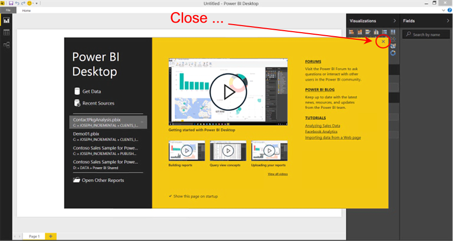
2. Click the “X” button in the upper right corner of the splash dialog that appears upon entry, atop the Power BI Desktop interface, as shown.

   Illustration 1: Close the Splash Dialog that Appears in Power BI

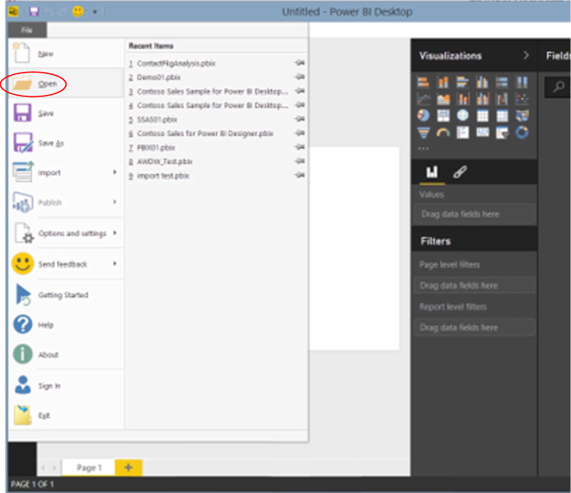
3. Select File - Open from the main menu.

   

   Illustration 2: Select File - Open in Power BI

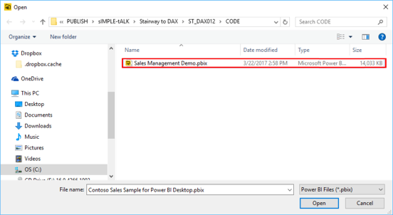
4. Locate and open the downloaded sample file, Sales Management Demo.pbix, from the Open dialog, as shown.

   Illustration 3: Select the Sample File …

5. Click Open.The .pbix file opens and we arrive within the Report view.
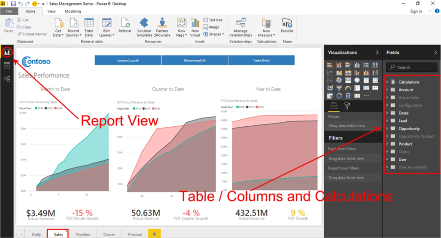
6. Click on the Sales tab (the second from the left at the bottom of the Report view).At this stage, we can see a few pre-configured reports, as well as the model’s member tables, etc., within the Fields pane on the right side of the desktop.

   Illustration 4: The Model Opens in Power BI Desktop (Sales Tab)

   Let’s leave the Report view (our current position in Power BI Desktop, which is indicated by the yellow bar that appears to the immediate left of the Report view icon), and look over the newly opened model from the tandem perspectives of Data and Relationships.

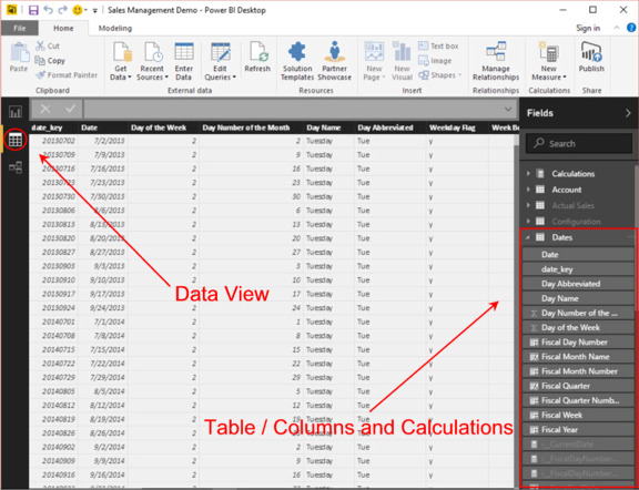
7. Click the Data view icon along the left of Power BI Desktop (the middle of the three icons).The data for one of the tables listed in the Fields pane on the right of the desktop appears below (in the immediate case, the Dates table’s data is partially displayed).

   Illustration 5: Power BI Desktop Data View

   We can examine each table, as well as add columns and calculations, within this and Report views as we’ll see throughout prospective Levels of this Stairway.

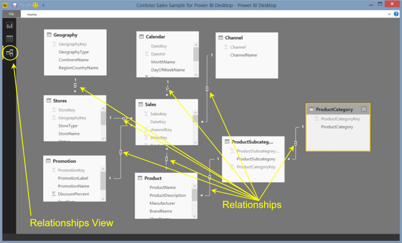
8. Click the Relationships view icon next, just below the Data view icon we last clicked.The schema, with relationships between tables, appears.

   Illustration 6: Relationships View

The CountA() Function

Introduction

According to the Microsoft Developer Network (MSDN), the DAX CountA() function “

counts the number of cells in a column that are not empty,” counting “not just rows that contain numeric values, but also rows that contain nonblank values, including text, dates, and logical values.”

CountA() is a member of the Aggregate functions group, whose members include Statistical and other functions, and which support common needs to create aggregations such as sums, counts, and averages. Many of these functions are very similar to counterpart aggregation functions used by Microsoft Excel.

CountA(), among many other DAX functions, as most of us are aware, is displayed as a selection in the Power BI Desktop Formula bar that appears when creating a new column or a new measure. The function is often used in combination with other DAX functions. CountA() is the first of the “A” functions that we have taken up in the Stairway to DAX and Power BI series. “A” functions are unlike “X” functions (which I introduced throughout the series) in that “A” functions employ only a single parameter, a column. Moreover, unlike the Excel CountA() function, with which many of us are familiar, the DAX version of CountA() accepts only a single argument. CountA() resembles the base Count() function found in DAX in most respects, but, like most “A” functions, differs from the base function in the fact that it is designed to handle non-date and non-numeric data.

NOTE: For an introduction to the DAX Count() and CountX() functions, see Stairway to DAX and Power BI - Level 8: Function / Iterator Function Pairs: The DAX Count() and CountX() Functions.

If we determine a need to extend the operation of CountA(), and take, as an argument, a column expression that is, in turn, evaluated for each row in a table, we can explore doing so via the CountAX() function (discussed in its own section of this Level below).

We will explore the syntax for the CountA() function after a brief discussion in the next sections. We will then gain some hands-on exposure to its use, within a practice example constructed to support a hypothetical business need in the Practice section later in this Level. This will allow us to activate what we explore in the Discussion and Syntax sections.

Discussion

DAX supports our needs to count rows or values with several functions (each of which we address within different Levels of this series). These include Count(), CountBlank(), CountRows(), and DistinctCount(), as well as CountA(). Among these, CountA() offers heightened flexibility, in that it can be applied to any column type and returns the number of values within the column that are not empty.

The CountA() function counts the number of ALL the cells in a column that are not empty; this includes not just rows that contain numeric values, but also rows that contain nonblank values, including text, dates, and logical values. When CountA() does not find any rows to count within a specification we give it, then it returns a blank. When there are rows, but none of them meet the specified criteria, then the CountA() returns a zero. CountA() can, like most DAX functions, be employed within other DAX functions.

Syntax

Syntactically, in using the CountA() function to count all non-blank cells in a column (numeric, text, date, logical – any except empty values), we specify the column containing the values to be counted to the right of the CountA keyword, as shown here:

  =COUNTA(<column>)

The returned value is a whole number. CountA() returns a zero when rows exist, but the values of those rows don’t meet the criteria we specify. The function simply returns a blank when it determines that there are no rows to count.

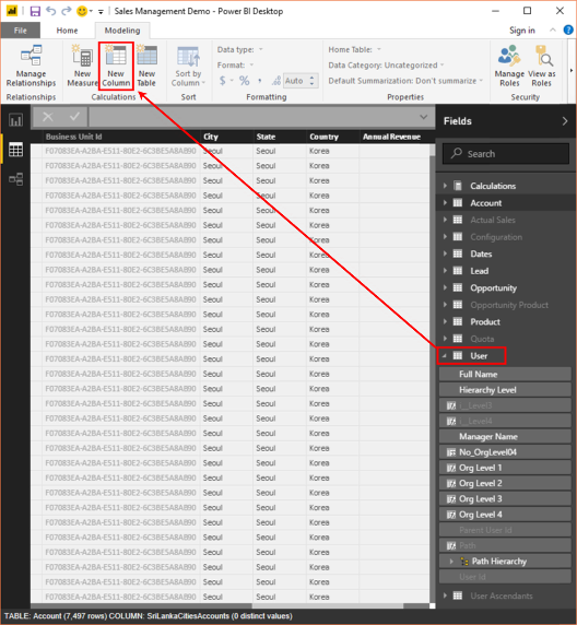
As an illustration, let’s take a look at a simple use of CountA(). We might wish, say, to do a “quick and dirty” count of users in Organizational Level 4 of the User table in the model. To do so, we could create a simple calculated column within the User table:

  No_OrgLevel04 = COUNTA('User'[Org Level 4])

Let’s say we’ve already employed CountA() in this way, via a simple calculation called No_OrgLevel04, within the Users table. The value of No_OrgLevel04 displays within the new column in the table in the Data view:

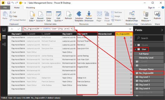
Illustration 7: Simple Example of the CountA() Function at Work

It doesn’t take much imagination to reach beyond the view we see above, where, for the sake of an easy example, we’re using the CountA() function to generate  the number of nonempty cells in a column to see how the calculation returns the desired outcome.

We’ll replicate this approach in the hands-on Practice section below, simply to enable easy verification of the accuracy of the results and so forth. Moreover, we’ll examine another, similar example with CountA() in the Practice sections below. Before we get to our practice with CountA(), let’s introduce its “X” partner, CountAX().

The CountAX() Function

Introduction

According to the Microsoft Developer Network (MSDN), the DAX CountAX() function “counts nonblank results when evaluating the result of an expression over a table.” In other words, CountAX() works just like CountA(), in that it returns a count of non-empty cells; the difference is that, while CountA() performs its count upon a specified column, CountAX() iterates through the rows of a table according to a specified expression that returns a nonempty result. CountAX() takes two arguments, the first of which must be a table, or any expression that returns a table. The second argument is an expression that is evaluated for each row of the specified table.

CountAX() is a member of the Aggregate functions group, as is CountA(), whose members include Statistical (which both CountA() and CountAX() are) functions among others and which support common requirements to create aggregations as we have already mentioned. CountAX(), like other iterator (“X”) functions, lends itself to use in combination with other DAX functions. CountAX() works like other iterator functions in its employment of a table expression (the first parameter specified within the function), for which a calculation, based upon an expression specified by a second parameter, is performed iteratively for each row of the table. The ultimate result is generated by the application of the CountAX() function to the dataset returned by the first and second expressions.

CountAX() counts the cells containing any type of information, including other expressions. As an illustration, if the column contains an expression that evaluates to an empty string, CountAX() treats the result as “nonblank.” It is important to keep in mind that, although CountAX() does not count empty cells, in a case like this one, the cell contains a formula, so it is counted. When the CountAX() function determines that there are no rows to aggregate, it returns a blank. Alternatively, if rows are found, but none of those rows meet the criteria we specify, CountAX() returns a zero.

We’ll briefly discuss CountAX() function specifics, and explore CountAX() from a syntax perspective in the sections that follow. Next, we’ll get some practical exposure to the use of the function within a practice example constructed to support hypothetical business needs, activating what we have explored in the Discussion and Syntax sections.

Discussion

As we have discovered, the CountAX() counts nonblank results when evaluating the result of an expression over a table. Let’s look at some syntax illustrations to further clarify the operation of CountAX(). We might think of CountAX() simply as a Count() function variant, where the “A” component is employed to enforce a count of values that are neither dates nor numerals, and where the “X” enforces counts across a specified table-column.

Syntax

The CountAX() function returns the result of an expression evaluated for each row in a table. The first argument is the table expression, and the second argument is the expression that we seek to apply to each row of the table returned by the first argument. The general syntax is shown in the following string:

  COUNTAX(<table>,<expression>)

Putting CountAX() to work is intuitive, particularly once we understand how CountA(), and “X” iterators in general, work, and once we grasp the purpose. Let’s take a look at a simple example in Power BI Desktop, this time via a calculated column we might add, and which we might place within a visualization.

Let’s say that we wish to know how many accounts we have in the data source that are 1) in Sri Lanka and 2) assigned to a specific city (we know of at least one “national level” account and want to exclude that from the count). To do so, we might, for purposes of a simple illustration, add a column within the Account table bearing a calculation like this:

  SriLankaCitiesAccounts = COUNTAX(FILTER('Account',Account[Country]="Sri Lanka"), Account[City])

Had we already made the insertion to the table, the numeric value of the new SriLankaCitiesAccounts accounts column would appear like this in the Data View:

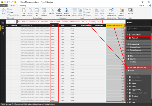
Illustration 8: Simple Example of the CountAX() Function at Work

We’ll observe a slightly more sophisticated example in the Practice section below, where we’ll see CountAX() used to a more practical purpose (and where we employ a measure, versus a column, which I would tend to do in most cases anyway, of course). Let’s get some hands-on practice with CountA() and CountAX() in the sections that follow.

Practice

To reinforce our understanding of the basics, we’ll put the CountA() and CountAX() functions to work within the step-by-step definition of some calculations. Our approach will be to do this somewhat as we have in the other Levels of this Stairway series: First, we’ll work with the functions via columns within the Data view of the model we have established. Then we’ll work with them via measures that we create, and then put to work within a straightforward visualization. The intent, as in all the practice sessions we undertake together within this series, is to demonstrate the operation of the functions we examine in an easy-to-understand, memorable manner. We will turn to the Power BI Desktop model we prepared earlier as a platform from which to construct and execute the DAX we examine, and to view the results we obtain.

Add a New Column in the Data View

We’ll begin, as noted, with a straightforward example: We’ll reconstruct the No_OrgLevel04 column we previewed earlier (see Illustration 7).

To recreate the No_OrgLevel04 column, we will take the following steps:

1. Return to the Data view.
2. Click the inward-pointing arrow, at the left of the User table, in the Fields list (on the right side of the Data view), to expose the table’s columns.
3. With the User table selected, click the New Column button on the Modeling tab of the ribbon, as shown.

   Illustration 9: Creating a New Column in the User Table …

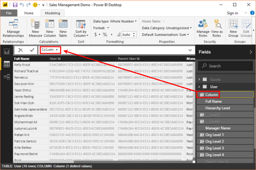
   The placeholder name of “Column” appears in the Formula bar, and among the User table columns, as depicted.

   

   Illustration 10: The Column Placeholder Appears …

4. Type the following DAX into the Formula bar, replacing the “Column = “placeholder:

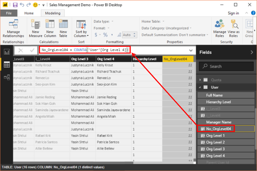
     No_OrgLevel04 = COUNTA('User'[Org Level 4])
   

5. Press the ENTER key.The new No_OrgLevel04 column replaces the placeholder in the Fields list and the column is populated in the Data view, as partially shown.

   Illustration 11: The No_OrgLevel04 Column is Populated (Partial View)

   The expected result, the count of the non-empty cells (“…not just rows that contain numeric values,” but all rows containing nonblank values …), appears in the Org Level 4.

   As we can see, CountA() is a straightforward function. Let’s create another calculation via the steps that follow.

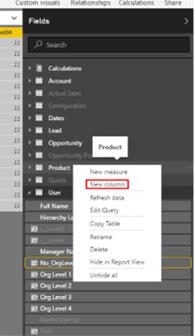
6. From where we are inside the Data view, locate, and right-click, the Product table in the Fields list.
7. Select New Column from the context menu that appears.

   Illustration 12: Select “New Column …”

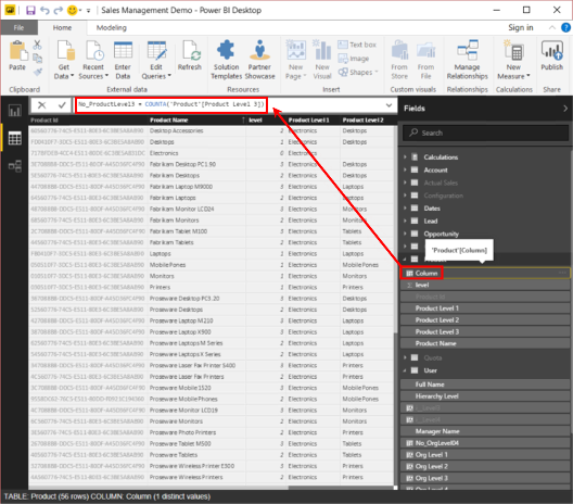
8. Type the following DAX into the Formula bar, replacing, as before, the “Column = “placeholder:

     No_ProductLevel3 = COUNTA('Product'[Product Level 3])
   

   

   Illustration 13: Adding the Calculation for the New No_ProductLevel3 Column …

9. Press the ENTER key.The new No_ProductLevel3 column replaces the placeholder in the Fields list and the column is populated in the Data view, as partially depicted.

   Illustration 14: The New No_ProductLevel3 Column is Populated (Partial View)

   We note that the new column is populated with the number 48. From the lower left corner of the Data View, we can see that the Product table contains 56 total rows. Let’s do a brief accuracy check on the number we have generated with CountA().

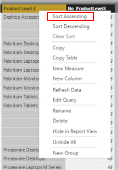
10. Right-click the header for the Product Level 3 column (to the immediate left of our new calculated column).
11. Select Sort Ascending from the context menu that appears.

    Illustration 15: Sort the Product Level 3 Column in Ascending Order

    The Product Level 3 column is sorted, with “empties” / nulls appearing at the top, as partially shown.

    

    Illustration 16: Eight Blank Rows Appear in the Product Level 3 Column

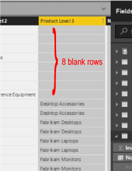
We can easily see that the “48” returned by our calculated column is correct: of the total 56 rows, COUNTA() has performed a count of all the rows in the Product Level 3 column that are not empty (there are eight blank rows). A count of 48 is correctly returned.

Putting a Simple Business Solution Together in the Report View

Now let’s get some hands-on exposure to CountAX() through a straightforward, “Report-view” example. Let’s say that our client, the Contoso organization, has asked us for guidance in their ongoing assembly of reports in Power BI: The immediate need is to create a measure that counts their customer Accounts (by name), which they intend (at least for starters) to use to report both total counts and accounts by customer account Country within a new dashboard. As they have asked us to help with the calculation, we’ll build a couple of simple visualizations to demonstrate basic uses for the calculation, which they can then reference to meet additional needs that arise later.

To meet the client requirements, let’s take the following steps:

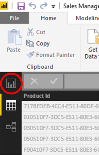
1. Click the Report view icon in the left navigation bar:

   Illustration 17: Go to the Report View in Power BI Desktop …

   We can check the tab marked with the “+” sign to the right of the existing tabs at the bottom of the report to arrive at a blank canvas. Here we will construct a calculation to meet the Contoso requirements. We’ll be able to construct a couple of visualizations while building the calculation those visualizations will contain – one of the conveniences of being able to access the model structure while within the Reports view.

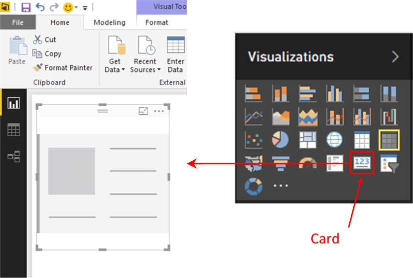
2. Click the Card visualization within the Visualizations pane.An empty Card visualization appears on the canvas.

   Illustration 18: Launch a Card Visualization on the Canvas (Composite Image)

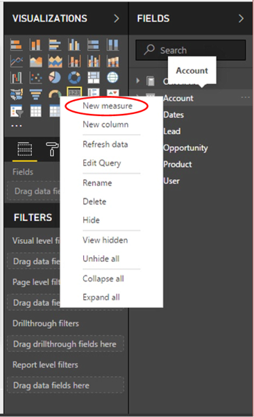
3. In the Fields list on the right of the desktop, right-click the Account table.
4. Select New Measure from the context menu that appears, as shown.

   Illustration 19: Select New Measure …

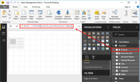
5. Type the following into the Formula bar of the Data view:# Accts = COUNTAX(Account,Account[Account Name])The measure definition appears in the Formula bar of the Report view as depicted:

   Illustration 20: Measure Using CountAX()

6. Click the checkmark icon to the left of the Formula bar to syntax check, and enter / save the new measure.We see the new measure created conveniently within the Report view, as discussed.
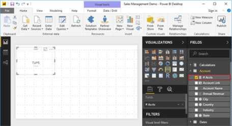
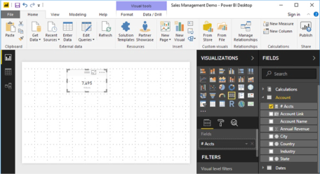
7. Ensuring that the Card visualization is selected on the canvas, click the check box to the immediate left of the new # Accts measure in the Fields pane.The card appears, with the total number of accounts calculation, on the Card, as shown.

   Illustration 21: Number of Accounts Appears on the Card Visualization

   Now let’s employ the measure in another visualization, in a way that we can validate the accuracy of our new # Accts measure. Our intent will be to display, within a Matrix, the total number of accounts that we see in the card, broken out by country.

8. Drag the newly created card to the right to make space for the next visualization we will be adding, something like this:

   Illustration 22: Making Room to Accommodate a Matrix …

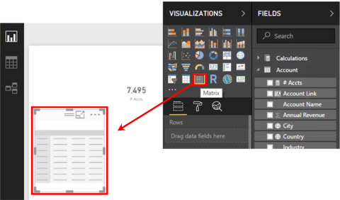
9. Click outside the existing card visualization, and then click the Matrix visualization inside the Visualizations collection to the right of the canvas.An empty Matrix appears on the canvas, as shown:

   Illustration 23: Adding a Matrix to the Canvas (Composite Image) …

10. Drag the Matrix toward the upper left corner of the canvas.
11. With the Matrix still selected, expand the Account table in the Fields section to the right of the Visualizations section.
12. Select the Country column that appears underneath the expanded Account table.The names of the Countries in which Contoso has accounts populate the rows of the Matrix, by default.
13. Select the # Accounts measure we created earlier, which also appears within the expanded Account table.The number of accounts appears to the right of each Country within the Matrix.

    Illustration 24: Matrix with Row and Value Selections (Composite Image)

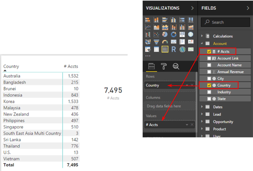
This simple example illustrates the operation of the CountAX() function, and how it respects context when used for the full population as in the Card above, as well as for the individual countries within the Matrix. It’s easy to see how the combination of the two visualizations affords a quick “reality check” of our calculation, which we were able to construct within the Report view as we have seen in practice exercises in the past. The capability to assemble and test all the pieces in one “studio” area like this can, of course, save significant time when we design solutions for more complex needs.

Summary …

In this Level of the Stairway to DAX and Power BI series, we explored the DAX CountA() and CountAX() functions. We discussed the respective purposes, syntax and operation of the two, and then focused upon using each in general. We also compared and contrasted ways that each can be employed, noting that we can combine them with other functions to achieve results like those we might need to deliver in client or employer environments.

In like manner to our standard approach to every DAX function we explore within the Stairway to DAX and Power BI series, we undertook illustrative examples of the uses of CountA() and CountAX() in practice exercises, and then observed the results datasets we obtained. We extended our exploration of CountA() and CountAX() to the delivery of illustrative answers to business questions, within both the data model and visualization levels of Power BI. In accordance with another objective of the series, we exposed practical examples of features of Power BI as a platform for employing DAX in our data models and visualizations to meet representative sample business requirements.