

Introduction to the DBScan algorithm
In this example, we are going to learn how to use DBScan. DBScan is a clustering algorithm used to find patterns. We are going to use it to analyze SQL Server data and find patterns about customers. In this tutorial, we will create Python code and connect to SQL Server, and analyze data.
Requirements for the DBScan
- SQL Server and SSMS installed.
- Visual Studio Code or another Python code editor of your preference.
- The AdventureworksDW2022 database installed.
- PyODBC library (pip install pyodbc)
- Pandas’ library (pip install pandas)
- Scikit-learn library (pip install scikit-learn)
- Matplotlib library (pip install matplotlib)
What is DBScan?
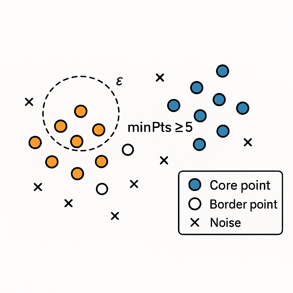
DBScan (Density-based spatial clustering of applications with noise) is a cluster algorithm based on density. It creates groups based on points that are closely packed. For this algorithm, you require the following information:
- ε (epsilon) is the neighborhood radius. This parameter is used to decide the closing points.
- MinPts is the minimum number of points within a radius.
- Core points are points that have at least minPts neighbors.
- Border points are within ε of some core points, but they are not close enough to the core.
- Noise are points outside ε and excluded from clusters
Getting started with DBScan
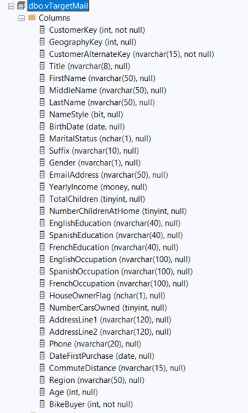
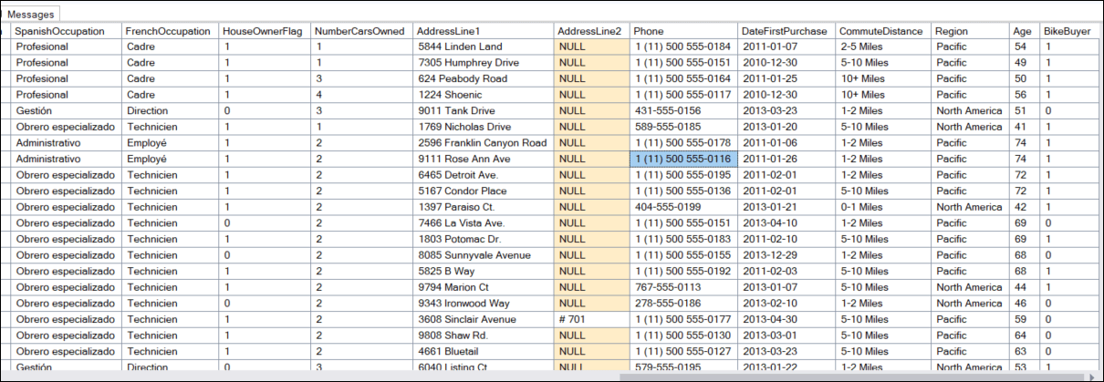
First, we will analyze the vTargetmail view of the AdventureworksDW2022 database. This table contains information about customers and potential customers, like Title, MaritalStatus, BirthDate, Gender, etc. The column bike buyer shows 0 if it is a bike buyer and 1 if it is not a bike buyer.
Here you have a sample of the data:
 Sample of data
With the DBScan algorithm, we will group the customer information in DBScan clusters using Python.
The Python code
Here is the code. We will show the entire code first, and then we will explain each section.
First, in Visual Studio Code or any Python core editor, write the following code:
import pyodbc
import pandas as pd
from sklearn.preprocessing import StandardScaler
from sklearn.cluster import DBSCAN
import matplotlib.pyplot as plt
# Connection to SQL Server (Windows Authentication)
conn = pyodbc.connect(
'DRIVER={ODBC Driver 17 for SQL Server};'
'SERVER=localhost;'
'DATABASE=AdventureWorksDW2019;'
'Trusted_Connection=yes;'
)
# Query relevant data
query = """
SELECT
[Age],
[YearlyIncome],
[TotalChildren],
[BikeBuyer]
FROM [dbo].[vTargetMail]
WHERE
[BikeBuyer] IS NOT NULL;
"""
df = pd.read_sql(query, conn)
conn.close()
# Inspect the data
print("First registers:")
print(df.head())
# Select the predictive characteristics
features = ['Age', 'YearlyIncome', 'TotalChildren']
X = df[features]
# Standarize the data (important for DBSCAN)
scaler = StandardScaler()
X_scaled = scaler.fit_transform(X)
# Apply DBSCAN
eps_value = 0.6
min_samples_value = 5
dbscan = DBSCAN(eps=eps_value, min_samples=min_samples_value)
df['Cluster'] = dbscan.fit_predict(X_scaled)
# Clusters summary and BikeBuyer proporcion
cluster_summary = df.groupby('Cluster')['BikeBuyer'].value_counts(normalize=True).unstack().fillna(0)
cluster_summary = cluster_summary.rename(columns={0: 'NoBuyer', 1: 'Buyer'})
print("\nProportion of BikeBuyer per Cluster:")
print(cluster_summary)
# Visualize clusters
plt.figure(figsize=(10, 6))
plt.scatter(df['Age'], df['YearlyIncome'], c=df['Cluster'], cmap='viridis', alpha=0.7)
plt.xlabel('Age')
plt.ylabel('YearlyIncome')
plt.title('Clusters of users - DBSCAN')
plt.colorbar(label='Cluster ID')
plt.show()
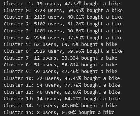
# Extra: quick summary per cluster
for cluster_id, group in df.groupby('Cluster'):
buyer_pct = group['BikeBuyer'].mean() * 100
print(f"Cluster {cluster_id}: {len(group)} users, {buyer_pct:.2f}0ought a bike")In the next section, we will explain the code.
Libraries used
First, to connect to Python, you need the pyodbc library. Secondly, see the requirements if you did not install it. This library is used to connect to SQL Server. Also, we have the Pandas library, which is used to read the SQL Data in a DataFrame. It will read the data.
In addition, we have the scikit-learn – StandardScaler library, which is used to standardize the data. In the code, the year's income could dominate distance calculations. scikit-learn – DBSCAN uses the DBSCAN algorithm. This library is the most important one. Finally, we have matplotlib.pyplot library is used to create the charts.
import pyodbc

import pandas as pd

from sklearn.preprocessing import StandardScaler

from sklearn.cluster import DBSCAN

import matplotlib.pyplot as plt
Connection to the SQL Server database
The second part of the code will connect to the SQL server. First, we will connect using Windows Authentication ('Trusted_Connection=yes). Secondly, we will specify the driver. The DRIVER is used to specify the ODBC Driver used to connect to SQL Server. Server is used to specify the SQL Server name. Also, we have the Database. Write the database name.
Finally, we have a query to get the data from the vTargetMail view.
# Connection to SQL Server (Windows Authentication)

conn = pyodbc.connect(

'DRIVER={ODBC Driver 17 for SQL Server};'

'SERVER=localhost;'

'DATABASE=AdventureWorksDW2019;'

'Trusted_Connection=yes;'

)


# Query relevant data

query = """

SELECT

[Age],

[YearlyIncome],

[TotalChildren],

[BikeBuyer]

FROM

[dbo].[vTargetMail]

WHERE

[BikeBuyer] IS NOT NULL;

"""
Read and standardize the data for the DBScan
In this section, we read the code from the query and close the connection.
df = pd.read_sql(query, conn)

conn.close()
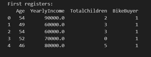
Secondly, we check a sample of the data.
# Inspect the data

print("First registers:")

print(df.head())
Thirdly, we select the input variables used in the model. X contains the dataframe with these values.
# Select the predictive characteristics

features = ['Age', 'YearlyIncome', 'TotalChildren']

X = df[features]
Also, we standardize the features. Standardization is used to put features on comparable scales. If one feature is bigger than others, the code puts them on comparable scales.
# Standardize the data (important for DBSCAN)

scaler = StandardScaler()

X_scaled = scaler.fit_transform(X)
Apply the DBSCAN
Now, we are going to use the DBScan algorithm. First, we need to use an eps_value. Secondly, we need the min_samples_value (MInPoints). As we explained before in the What is DBScan section, the Epsilon (eps_value) value is the neighborhood radius. It controls how far the algorithm looks to find the neighboring points.
The MinPoints or min_samples control the number of neighbors required for a cluster. Finally, it creates a cluster id for each cluster detected.
# Apply DBSCAN

eps_value = 0.4 # based on your k-distance

min_samples_value = 5

dbscan = DBSCAN(eps=eps_value, min_samples=min_samples_value)

df['Cluster'] = dbscan.fit_predict(X_scaled)
Cluster Summary for DBScan
In this section, you are determining which individuals are bike buyers and which are not. First, you group the data to remove the noise.
# Clusters summary and BikeBuyer proportions

cluster_summary = df.groupby('Cluster')['BikeBuyer'].value_counts(normalize=True).unstack().fillna(0)
Secondly, we are replacing the values 0 and 1 with the values of NoBuyer and Buyer.
cluster_summary = cluster_summary.rename(columns={0: 'NoBuyer', 1: 'Buyer'})Then we are displaying the proportion per cluster.
print("\nProportion of BikeBuyer per Cluster:")

print(cluster_summary)
Visualize the DBScan clusters
Finally, we will create a scatter chart with the DBScan cluster information. First, we will plot and send the Age and Yearly Income from the data file, and create a file with the viridis colors. Alpha = 0.7 means that the chart will be 70 percent opaque and 30 percent transparent. Secondly, we will plot Age on the x-axis and Yearly Income on the y-axis. Xlabel and ylabel will name the axis.
# Visualize clusters

plt.figure(figsize=(10, 6))

plt.scatter(df['Age'], df['YearlyIncome'], c=df['Cluster'], cmap='viridis', alpha=0.7)

plt.xlabel('Age')

plt.ylabel('YearlyIncome')

plt.title('Clusters of users - DBSCAN')

plt.colorbar(label='Cluster ID')

plt.show()
Extra summary per DBScan cluster
Also, this summary shows the cluster and the percentage of buyers per cluster. It will provide the percentage of buyers and not buyers.
# Extra: quick summary per cluster

for cluster_id, group in df.groupby('Cluster'):

  buyer_pct = group['BikeBuyer'].mean() * 100

  print(f"Cluster {cluster_id}: {len(group)} users, {buyer_pct:.2f}0ought a bike")
Running the DBScan code
Run the code and you will see the results. First, you will see a sample of the data.
Secondly, you will have the clusters and the proportion of buyers and non-buyers per cluster.
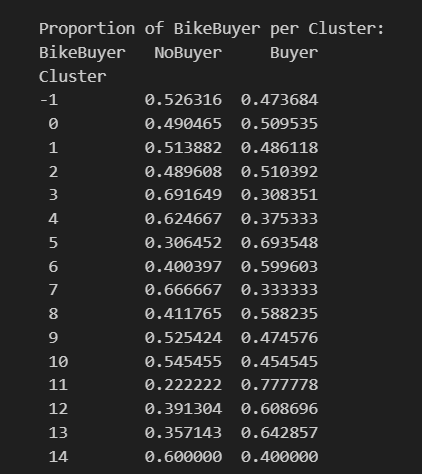 Proportion of bike buyers with DBScan
In addition, you will have the scattered chart of the Yearly Income and the Age. The clusters 12 to 14 belong to the people with a high income of more than 140,000 USD. There is also a small portion of a cluster with an age of around 100 years old and a low income below 2,000 USD.
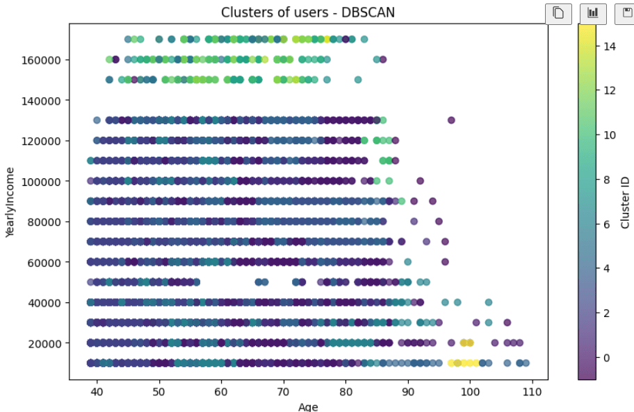 DBSCAN Chart
As you can see, the clusters in this example are mixed; it is not clear.
Finally, we have some statistics of people who bought a bike per cluster.
Conclusion
DBScan is a cluster algorithm that can be used to create clusters of data to detect anomalies and group the data to find patterns.
For more information about DBScan refer to the following links: