I’ve always wondered how SQL Server picks the column order in suggested indexes, and recently ran into a situation I just could not resist testing. Consider the following query:
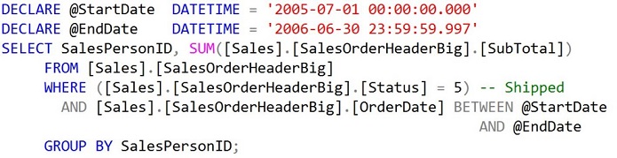
Figure 1: Baseline Query
This is from AdventureWorks2012Big. AdventureWorks2012Big is derived from AdventureWorks2012 using a script by Jonathan Kehayias, available at http://sqlskills.com/blogs/jonathan. This script adds two new tables (Sales.SalesOrderHeaderBig and Sales.SalesOrderDetailBig) and increases SalesOrderHeader from 31,465 rows to 1,290,065 rows. Actually upon investigation (after I finished the original draft), I found the for both the Sales.SalesOrderHeader and Sales.SalesOrderHeaderBig tables, the column, Status, only contained the value 5 for every row. After a review of random number generators, I modified the Sales.SalesOrderHeaderBig table's Status column to have roughly equal number of Status ranging from 0 to 9. This is probably closer to real world table data. You can find the code to do this in the attached SQL file.
This query is a typical report aggregate query where the WHERE clause is based on the Status and OrderDate columns. If I run this query with the original defined adventureWorks2012Big indexes, as shown in the query plan below, we get a Clustered Index Scan on SalesOrderHeaderBig where the Primary Key/Clustered Index is based on SalesOrderID (identity column):
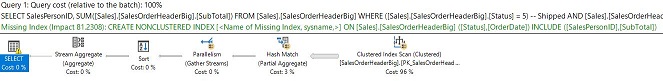
Figure 2: Query Plan with original indexes
This has:
- query cost = 22.9441
- logical reads = 30,311
- cpu = 173ms
Note that the suggested nonclustered index is defined on Status,OrderDate with SalesPersonID,Subtotal in the INCLUDE clause. This got me to thinking why isn’t OrderDate first. We all know (from Word of Mouth, WOM) that you should have the most selective column first.
So, if I define the new covering index (as suggested):
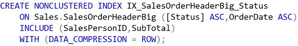
Figure 3: Microsoft Sugested Covering Index
The query optimizer didn't recommend the Data_Compression option, but from one of my previous blogs I know this is a best practive for almost all indexes -- clustered and non-clustered
And rerunning the same query, we get the following results:
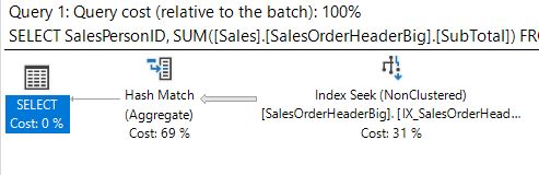
Figure 4: Query Plan with Nonclustered Index seek based on Status,OrderDate
This query now has:
- query cost = 0.563195
- logical reads = 12
- cpu = 0ms
Wow; a factor of 40 improvement in performance (query cost)! The covering index now gives us an index seek. But I am still wondering about the order of the index defining columns. So, let’s drop the new index and redefine a new one based on OrderDate,Status as shown below:
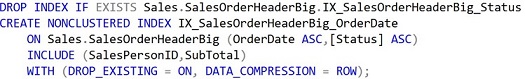
Figure 5: Revised Nonclustered Index based on OrderDate,Status
And rerunning the same query again. We now get
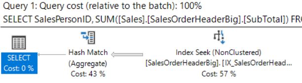
Figure 6: Query Plan with Nonclustered Index based on OrderDate, Status
This query now has:
- query cost = 1.14707
- logical reads = 72
- cpu = 15ms
We still get an index seek, but the statistics IO and Time are slightly worse and the query plan cost is slightly higher. The Index Seek cost jumped from 31 to 57% of the total query cost. Why is that?
If we go back to the query plan and hover the mouse cursor over the Index Seek operator in the respective query plans for the 1st, 2nd and 3rd queries we get:
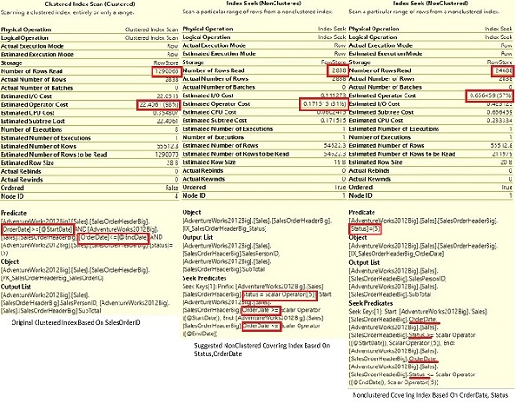
Figure 7: Index seek Query Plan properties for Index Scan and NonClustered index seeks (in order)
Interesting results can be derived from the three queries. Major difference shows up in the first query with the clustered index scan where each table row is checked for the OrderDate range and status = 5 resulting in 30,311 logical reads (Predicate). In the second query (recommended Microsoft non-clustered covering index) you only have a Seek Predicate and in the 2nd index scan query you have both a Seek Predicate and a Predicate.
So what’s the difference between the Seek Predicate and Predicate in the operator window? The Seek Predicate assists with the data recovery filtering the rows within the respective index (acts almost like a WHERE clause). The Predicate then eliminates the subsequent rows with the specified criteria. So even though there is just one operator here, the Seek Predicate filters the row during the data reads and the Predicate then filters the resulting interim row set. So in the original clustered scan, there is no Seek Predicate because each row much be accessed. The Predicate then filters the interim result set based on OrderDate and Status.
In the 2nd query using the suggested covering index there is only a Seek Predicate. The optimizer is taking advantage of the fact that given a Status of 5, the OrderDates are arranged in ascending order within the index. This is not the case for the nonclustered covering index based on OrderDate and Status respectively. In this case there is a convoluted “WHERE” clause on OrderDate and Status followed by a subsequent filtering just on Status = 5. This then results in the 2nd query having only 12 logical reads whereas the 3rd query because of the double filtering has 72 logical reads.
The above paragraphs will probably generate considerable discussion, and I look forward to that as I am in a continual learning mode.
So what happens if I go back and push the OrderDate down to the INCLUDE clause in IX_SalesOrderHeaderBig_Status as shown below (there is some index cleanup as indicated):
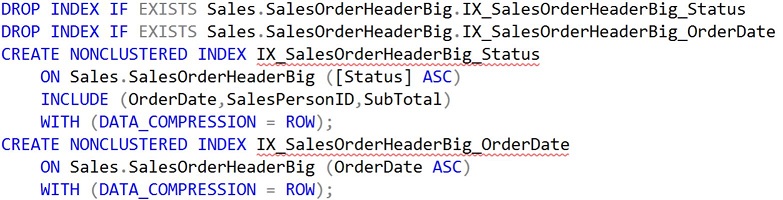
Figure 8: Push OrderDate down to INCLUDE clause
This new index retains the same columns as the original suggested index, but does not allow the optimizer to take advantage of ordering of OrderDate. Rerunning same query we get
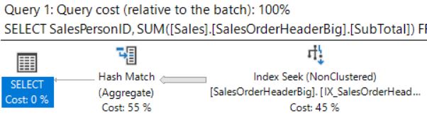
Figure 9: Query Plan with Nonclustered Index based on Status
This query now has:
- query cost = 0.919195
- logical reads = 367
- cpu = 31ms
If we hover over the Index seek operator we get
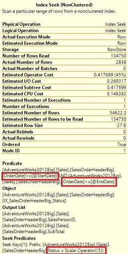
Figure 10: Index seek Query Plan properties for third index definition
Again we have the break out of Predicate and See Predicate, but now the Seek Predicate is based only on the Status Column and the Predicate on the Order column. In this case performance is better than the original clustered index scan, but just short of the suggested covering index.
Many times in my SQL Saturday Index presentations I have been asked what columns to retain in the index definitions. I usually give the standard Microsoft answer, “It Depends!”, but for these cases it really does depend on the data and scenario and whether or not the optimizer can take advantage of the ordering of the second (and maybe the third if applicable) column.
The overall results initially seemed counter-intuitive to me as I thought OrderDate was the more selective column. But apparently the ordering of OrderDate in the optimizer suggested index resulted in less logical reads as indicated. In any case, all three non-clustered covering indexes resulted in improved performance (less logical reads) than the original Clustered Index scan. But, just because you build a covering index, doesn’t necessarily mean it is the best. Testing should always be part of your regimen before deploying to production.
There also may be a few comments about my DATA_COMPRESSION = ROW parameter in the definition of the three indexes. In my experience and from my blog on data compression (https://logicalread.com/sql-server-index-compression-mb01/#.XFc0UPZFxPY) there are many benefits and almost no cons for using row data compression since data is compressed all the way from the hard drive to the buffer cache to the L3 processor cache and finally compressed/decompressed at the L2 cache of the processor. Data compression has been available from SS2008 Enterprise Edition and now available from SS2016 SP2 Standard Edition on.
Stay tuned for Part 2 where we look at how the definition of the clustered index affects the same query. We'll look at the original clustered index on an identity column and then look at the effect of a composite index based on the OrderDate column and the identity column.
Mike