

What is a metadata driven pipeline? Wikipedia defines metadata as “data that provides information about other data.” As a developer, we can create a non-parameterized pipeline and/or notebook to solve a business problem. However, if we must solve the same problem a hundred times, the amount of code can get unwieldly. A better way to solve this problem is to store metadata in the delta lake. This data will drive how the Azure Data Factory and Spark Notebooks execute.
Business Problem
Our manager has asked us to create a metadata driven solution to ingest CSV files from external storage into a Microsoft Fabric one lake. How can we complete this task?
Technical Solution
We are going to go back to the drawing board for this solution. First, we have determined that the CSV files stored in the ADLS container are small to medium in size. Second, we are going to keep historical files around for auditing in the bronze layer. Third, the silver layer will present to the end users the most recent version of the truth (data). Since the datasets are tiny in nature, we are going to use a full load process.
The following topics are investigated in this article.
- create a metadata table
- populate metadata table
- create a data pipeline
- create credentials for storage
- create parameters and variables
- code for a copy activity
- code for notebook activity
- evaluate 3 use cases
- any future enhancements
Architectural Overview
The architectural diagram for this metadata driven design is seen below.
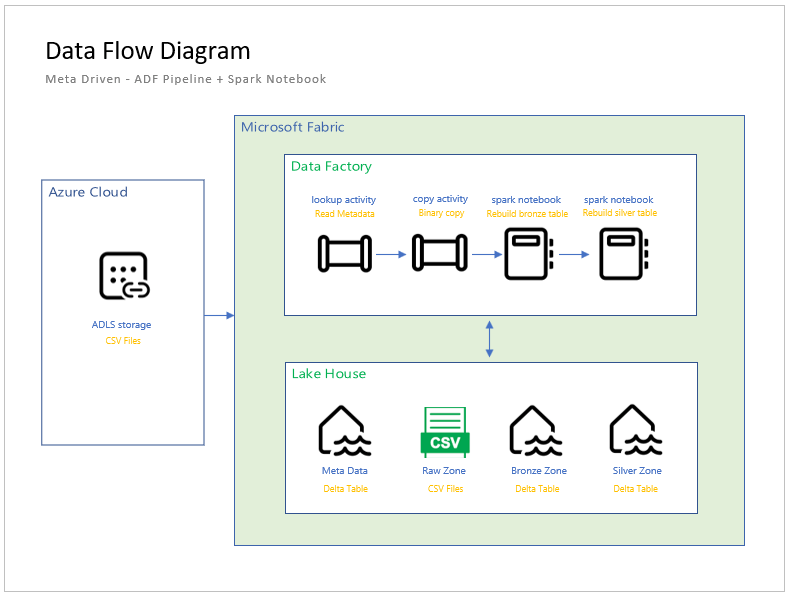
There are three major components: Azure Data Lake Storage which is external to the Fabric service; Data Factory Pipeline Activities that read/write files; and the Lake House storage with its medallion layers. Please note that medallion layers are either folders and/or naming conventions to organize the data in logical buckets.
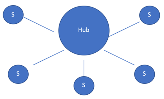
A popular use case of a data lake is to collect data from various disconnected systems (producers) and place the data into single location (hub). However, there are always users (consumers) that want to access the data using their favorite tools. That is why a data lake is considered a spoke and hub design.
As a Microsoft Fabric designer, we can use either data pipelines or data flows to move the data into the lake. I chose pipelines since they can be easily parameterized. At the transformation layer, we must choose between Spark notebooks or data flows. Again, I decided to pick notebooks since the code is portable to other platforms. Since the SQL endpoint does not support Spark views, we are going to have to add this gold layer using data warehouse views.
Meta Data Tables
A meta data driven design allows the developer to automate the copying of data into the lake (raw files) as well as building the bronze and silver tables. The image below shows the meta data table viewed from the SQL endpoint.
This is a spoiler alert. Since the gold tables are usually custom for each lake, we will be talking about Synapse Data Engineering and Data Warehouse design in our next article.
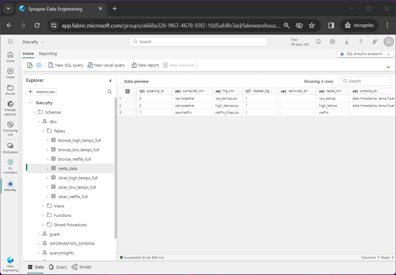
The above image shows the end state of our article. The Netflix, high temperature and low temperature raw files have been converted to both bronze and silver tables.
Let us focus on the meta data table right now with the following fields.
- pipeline id – just an identifier
- container name – same path in source and destination storage
- file name – same file in source and destination storage
- header flag – does the data file have a header line
- delimiter string – how is the tuple divided into columns
- table name – the root name of the table
- schema string – infer schema or use this definition
The purpose of this section is to show the developer how to drop tables, create tables, and insert data. These actions are required to create our meta data table and populate it.
%%sql
--
--  remove table
--


drop table if exists meta_data;
The above Spark SQL drops the meta data table, and the below SQL code creates the table.
%%sql
--
--  create table
--


create table meta_data
(
  pipeline_id int,
  container_nm string,
  file_nm string,
  header_flg boolean,
  delimiter_str string,
  table_nm string,
  schema_str string
);
Insert meta data for the Netflix dataset.
%%sql
--
--  netflix dataset
--


insert into meta_data values
(1, 'raw/netflix', 'netflix_titles.csv', true, ',', 'netflix', '');
Insert meta data for the high temperature dataset.
%%sql
--
--  weather - high temp dataset
--
insert into meta_data values
(2, 'raw/weather', 'high_temps.csv', true, ',', 'high_temps', 'date timestamp, temp float');
Insert meta data for the low temperature dataset.
%%sql
--
--  weather - low temp dataset
--

insert into meta_data values
(3, 'raw/weather', 'low_temps.csv', true, ',', 'low_temps', 'date timestamp, temp float');
Right away, we can see that will want a gold view to join the silver high and low tables into one logical dataset. This is not an uncommon request. I have a current client that has an old and new payroll system. In the data lake, they want one view of the payroll register. Thus, the view unions several tables into one logical one.
Azure Data Lake Storage
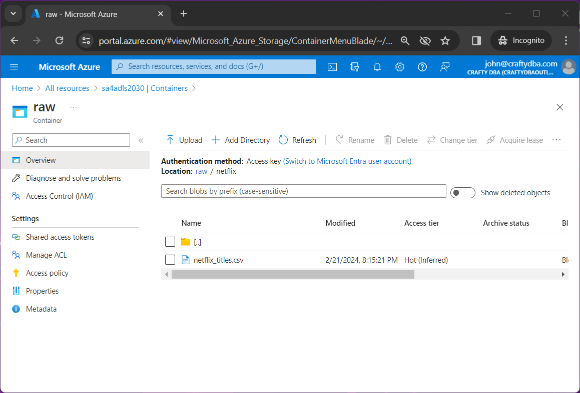
At this time, Microsoft Fabric does not support a on premise gateway. Use this link to find out the major differences between Azure Synapse and Microsoft Fabric in regards to data factory. In our proof-of-concept example, datasets will be dropped into an external storage account.
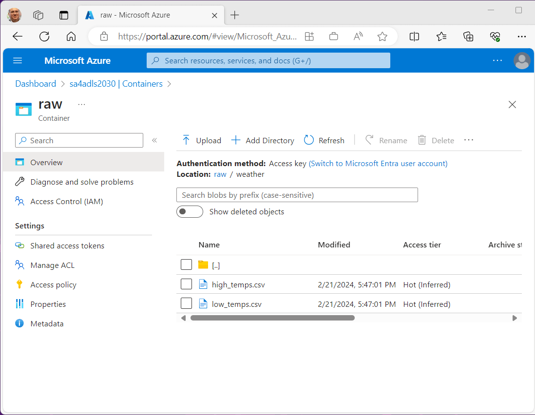
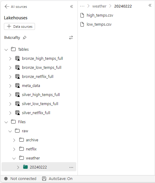
To make life easy, the container and path will be the same between the source and destination. The above image shows two temperature files, and the below image shows one Netflix file.
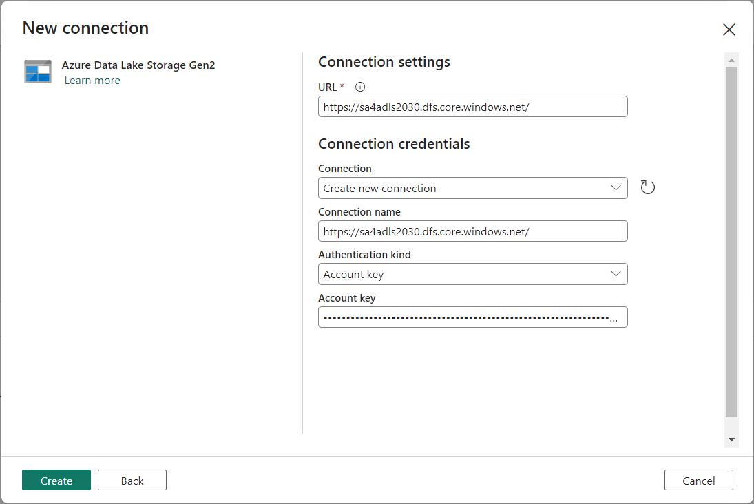
To simply the example, we are going to use an account key to access the Azure Storage Account.
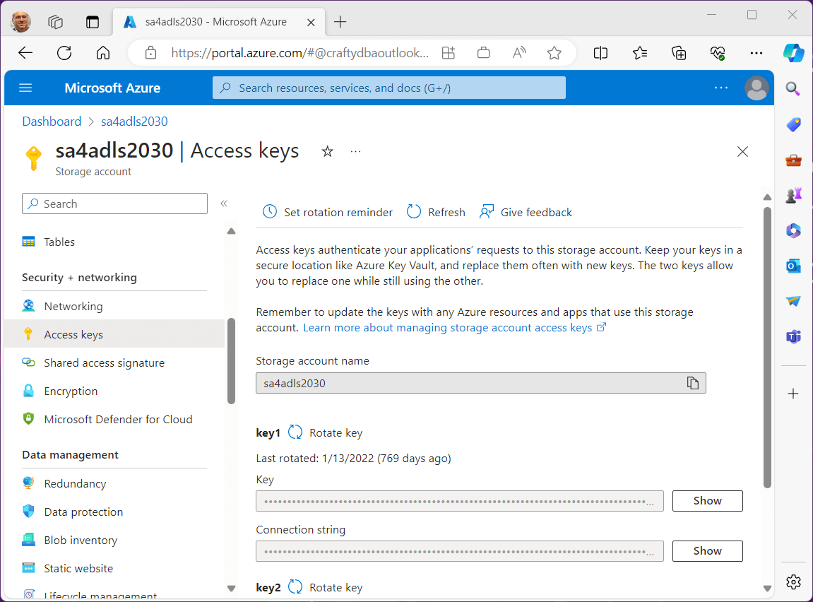
For a production system, I wound use a service principle since we can restrict access using both RBAC and ACL security.
In the next section, we are going to start building our data pipeline.
Data Pipeline – Copy Activity
Click the create icon on the left menu to start our Data Factory adventure. Both Data Flow and Data Pipelines are available to the developer. Please create a new Data Pipeline.
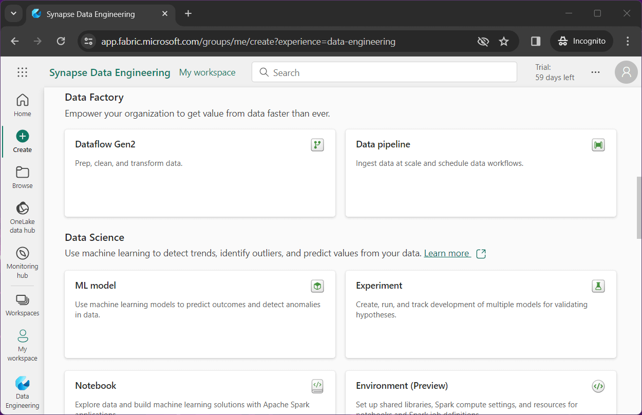
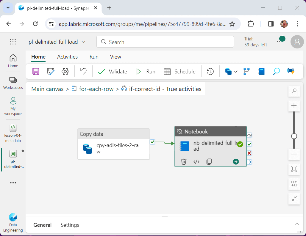
I am going to highlight the two activities that are key to our program. The copy activity allows a developer to read data from the source and write data to the destination. The notebook activity allows us to call a spark notebook that will tear down and rebuild the bronze and silver tables.

Let us work on the connection next. In prior versions of data factory, the developer created a linked service that contained the connection information and a dataset that described the data. For example, a linked service named ls_asql_hris, has the connection to an Azure SQL database and a dataset, named ds_asql_employee, describes the fields in the table.
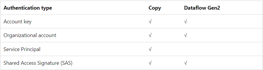
These two objects are replaced by one connection object in Fabric. The image below shows the support for many types of connections. We want to setup on for Azure Data Lake Storage.
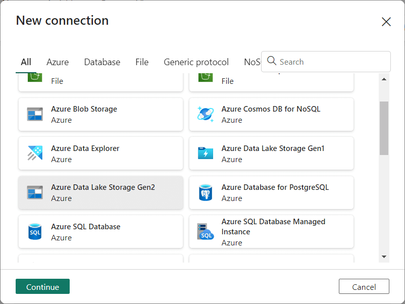
Supply the fully qualified location to the storage as well as the account key.
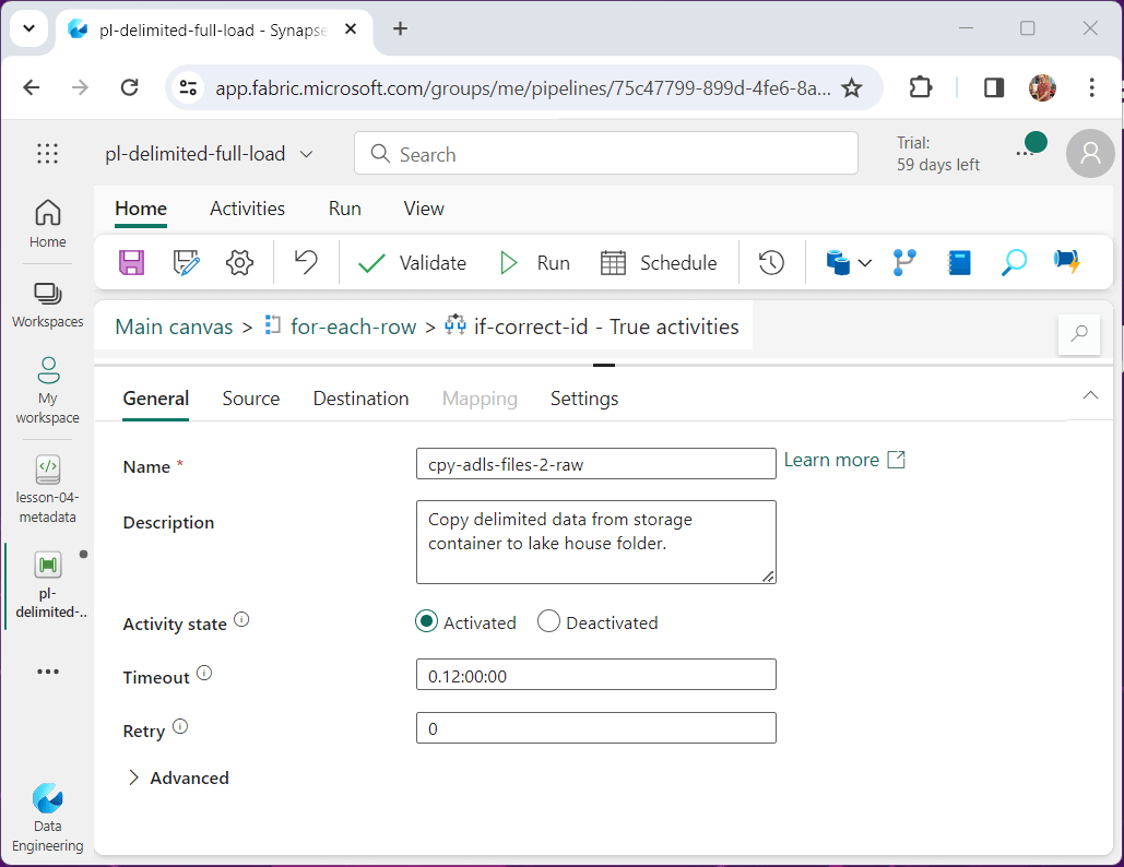
It is important to following your companies’ naming conventions for activities and add detailed comments when possible. The image below shows the copy activity we are about to configure.
Since we are only copying the file from the source to the destination storage, please choose a binary copy. The image below shows the container name and file name are parameters to the source definition.
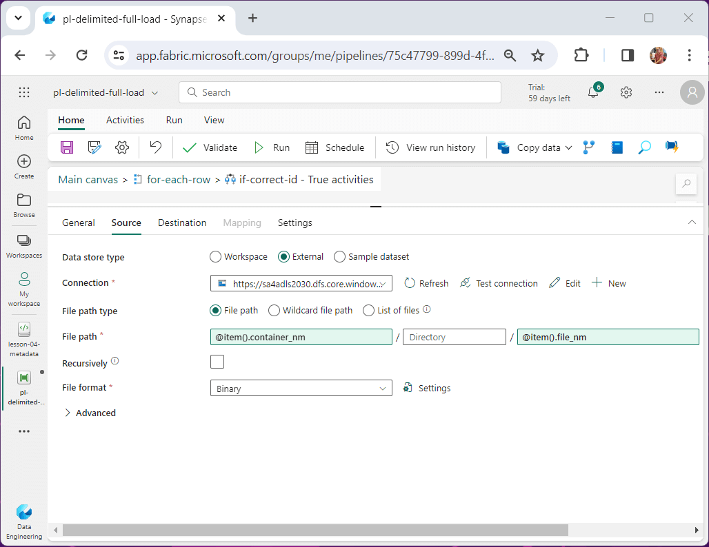
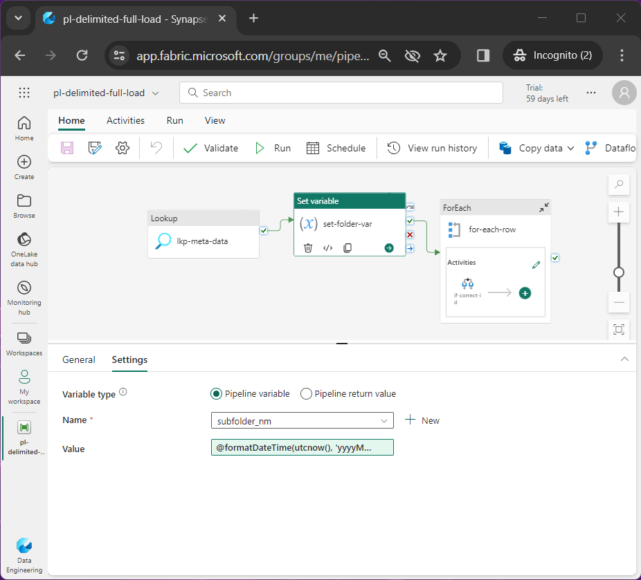
The same parameters are used for the destination with one addition. We are going to add the current date formatted as “YYYYMMDD” as a subfolder. That way, we can have multiple versions of the source files by a given day.
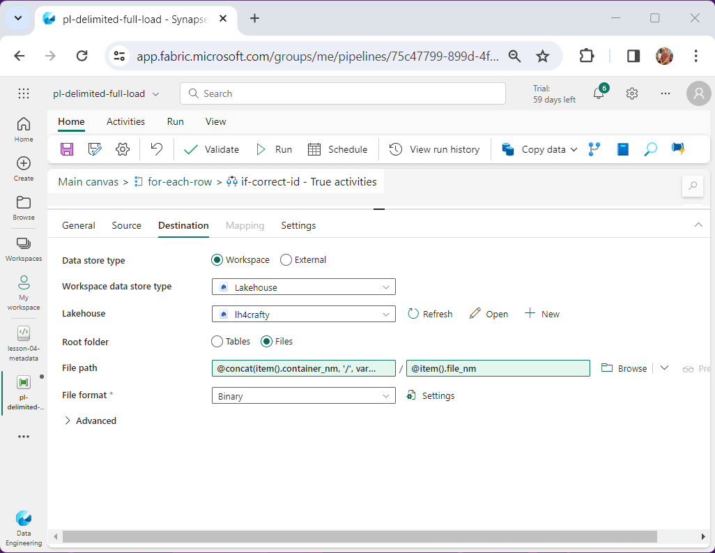
The item() variable is exposed to the activity when a for-each activity is used. We will talk about working with meta data using the lookup activity next.
Data Pipeline – Lookup & ForEach – Activities
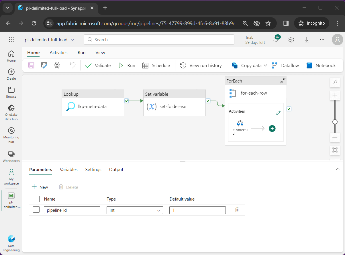
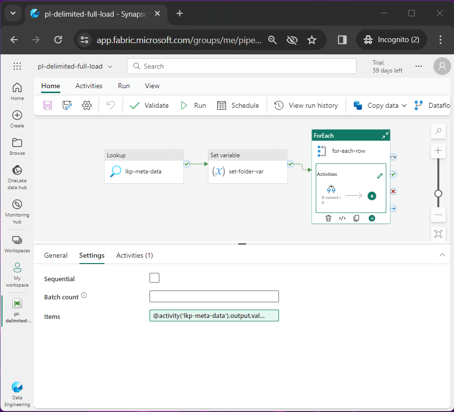
The image below shows the top three activities used by our data pipeline. The for-each activity has two levels of nesting. Please note I renamed the pipeline to pl-delimited-full-load and gave it an appropriate description. I defined a pipeline parameter named pipeline_id which tells the pipeline which row of meta data to use.
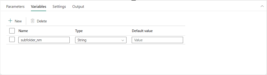
The variable shown below was used in the destination section of the copy activity.
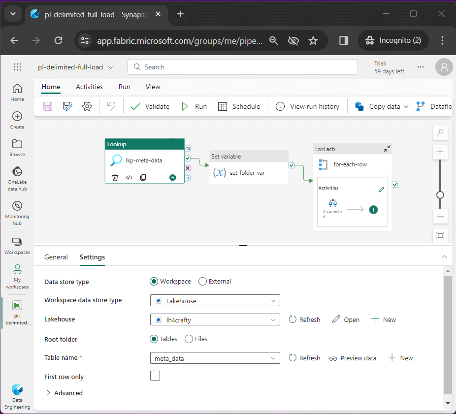
Let us review the details of the three topmost activities. The image below shows the lookup activity named lkp-meta-data reads the meta_data table from the lake house and returns a JSON object.
The set variable activity named set-folder-var converts the current data/time into a pattern for the creation of the sub-folder in our destination storage.
The for-each activity traverses the array of meta data records. The JSON output from the lookup activity is feed to the for-each activity as input.
The simplest way to execute the copy and notebook activity for the correct pipeline id is to use an if condition activity.
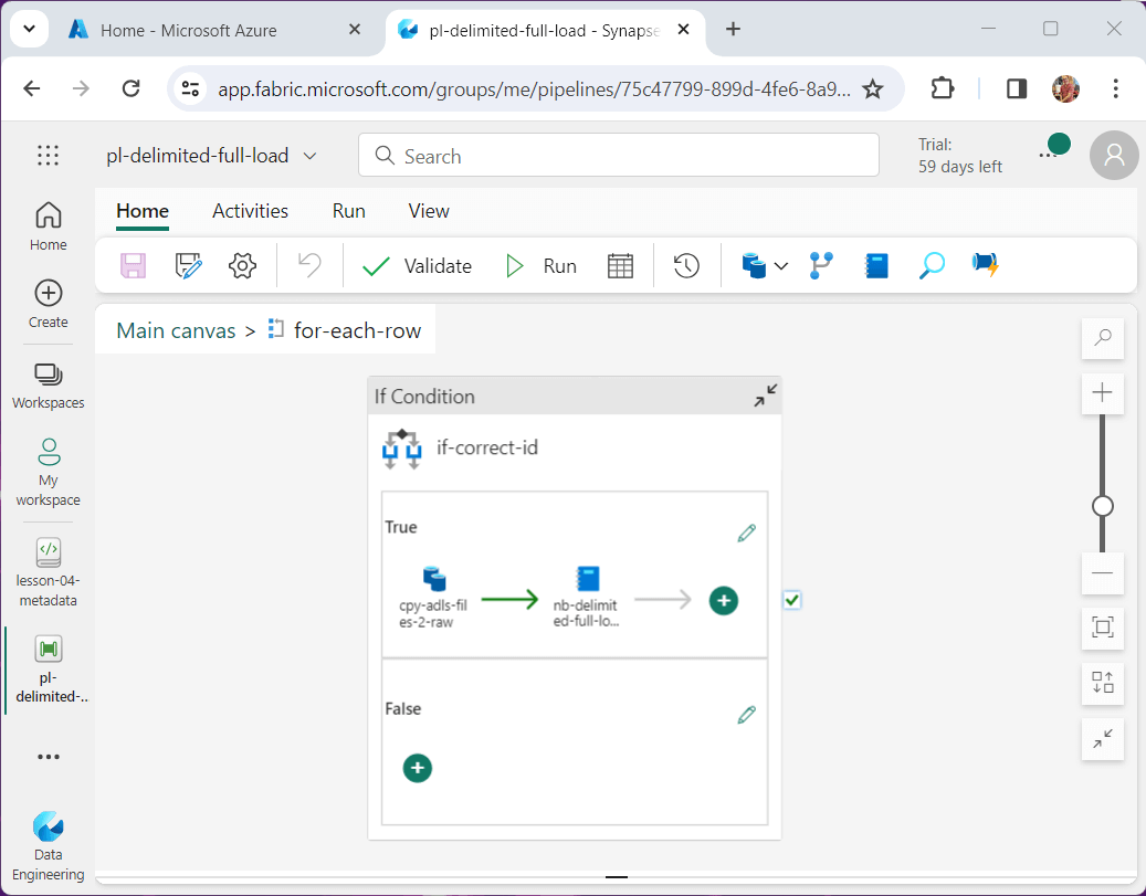
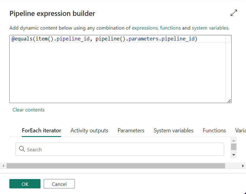
The details of the condition are shown below.
I usually do not repeat screen shots; However, this new feature in Data Factory is awesome!
When testing each component of a pipeline, the developer might want to de-activate or activate a component. I learn about this feature in the sequence container when developing packages in SSIS 2005. I am glad the feature made it to Data Factory.
To sum up this section, the lookup and for-each activity are really made for each other. We could make this code more complex by figuring out if the JSON output from the lookup activity has an array element that matches our pipeline id. However, all “if condition” tests are being done in parallel and it is not worth the effort to save a few seconds.
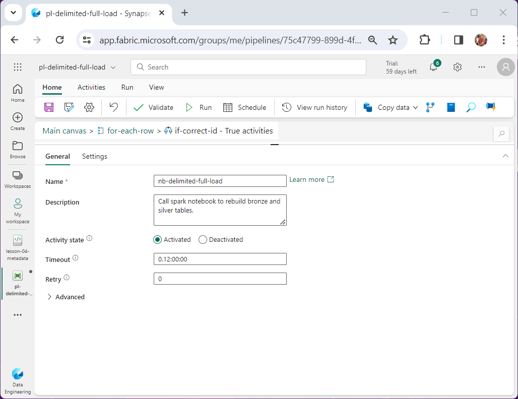
Data Pipeline – Notebook Activity
The notebook activity just calls the Spark Notebook with the parameters we supply. Please use a naming convention and enter detailed comments.
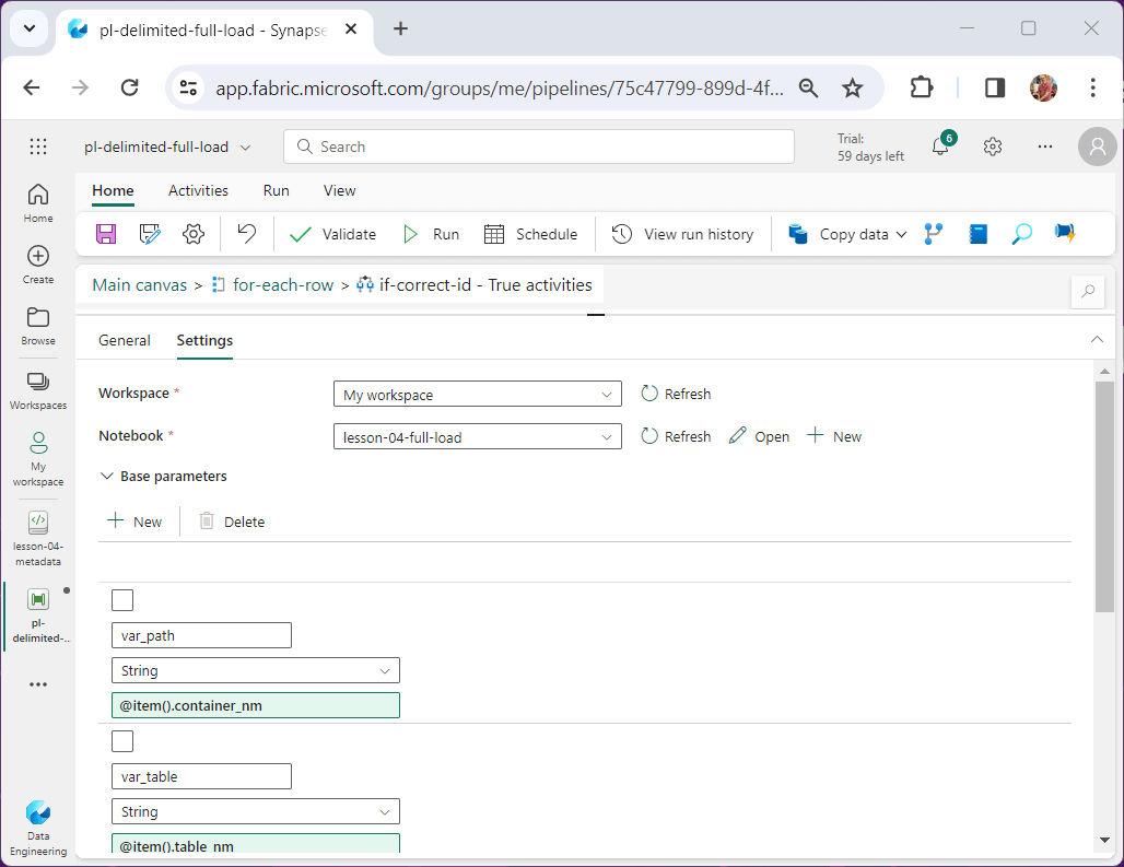
On the settings page of the activity, we browse the workspace for the notebook we want to run. In our case, the name of the notebook is lesson-04-full-load. The parameters match one for one to the fields in the meta data table.
Before we execute the finalized pipeline, let us look at the revised Spark Notebook.
Spark Notebook
At the top of the notebook, we need a header to describe the program as well as a parameter cell. The code below shows the parameter cell.
var_path = 'raw/netflix'
var_table = 'netflix'
var_delimiter = ','
var_header = 'true'
var_schema = ''
The first step of the notebook is to remove the existing bronze and silver tables for a given parameterized table name.
#
#  F1 - remove existing tables
#


# drop bronze table
stmt = f'drop table if exists bronze_{var_table}_full;'
ret = spark.sql(stmt)


# drop silver table
stmt = f'drop table if exists silver_{var_table}_full;'
ret = spark.sql(stmt)
The second step of the notebook is read the CSV file into a DataFrame and produce a temporary view as the final output. Two tests are performed on the schema variable. If the variable is None or an empty string after trimming, then we want to read infer the schema.
This code performs a full load – reading the file and creating temp view
#
#  F2 - load data frame
#


# root path
path = 'Files/' + var_path


# tmp table
table = 'tmp_' + var_table.strip() + '_full'


# schema flag
schema_flag = True


try:

  # none test
  if var_schema is None:
    schema_flag = False

  # empty string
  if not bool(var_schema.strip()):
    schema_flag = False

except:
  pass


# load all files w/o schema
if not schema_flag:
  df = spark.read.format("csv")
    .option("header",var_header)
    .option("delimiter", var_delimiter)
    .option("recursiveFileLookup", "true")
    .load(path)


# load all files w/ schema
else:
  df = spark.read.format("csv")
    .schema(var_schema)
    .option("header",var_header)
    .option("delimiter", var_delimiter)
    .option("recursiveFileLookup", "true")
    .load(path)


# convert to view
df.createOrReplaceTempView(table)


# debugging
print(f"data lake path - {path}")
print(f"temporary view - {table}")
The third step in the program creates the bronze table while adding a load date, a folder name, and a file name. The split_string function is called with parameters specific to our directory structure.
#
#  F3 - create bronze table (all files)
#


# spark sql - assume 1 level nesting on dir
stmt = f"""
  create table bronze_{var_table}_full as
  select
    *,
    current_timestamp() as _load_date,
    split_part(input_file_name(), '/', 9) as _folder_name,
    split_part(split_part(input_file_name(), '/', 10), '?', 1) as _file_name
  from
    tmp_{var_table}_full
"""


# create table
ret = spark.sql(stmt)


# debugging
print(f"execute spark sql - \n {stmt}")full load – create bronze table
The fourth step creates the silver table by only showing the data from the newest sub-directory by date string.
#
#  F4 - create silver table (lastest file)
#


# spark sql
stmt = f"""
  create table silver_{var_table}_full as
  with cte_{var_table} as
  (
    select *
    from bronze_{var_table}_full as l
    where l._folder_name = (select max(_folder_name) from bronze_{var_table}_full)
  )
  select
    *
  from
    cte_{var_table}
"""


# create table
ret = spark.sql(stmt)


# debugging
print(f"execute spark sql - \n {stmt}")
If this was a production system, I would be logging the record counts into an audit table. Here is code to print record counts for the bronze table.
#
#  Grab bronze count
#


try:
  sql_stmt = f"select COUNT(*) as Computed from bronze_{var_table}_full"
  bronze_recs = spark.sql(sql_stmt).first()[0]
except:
  bronze_recs = 0


# show values
print(f"The bronze_{var_table}_full record count is {bronze_recs}")
Of course, we want to show record counts for the silver table.
#
#  Grab silver count
#


try:
  sql_stmt = f"select COUNT(*) as Computed from silver_{var_table}_full"
  silver_recs = spark.sql(sql_stmt).first()[0]
except:
  silver_recs = 0


# show values
print(f"The silver_{var_table}_full record count is {silver_recs}")
Now that will have a complete Data Pipeline – copy data into lake and Spark Notebook – transform files into tables, lets execute the pipeline three times with each pipeline id to load the CSV files into our one lake (lake house).
Testing
Please set the pipeline variable named pipeline id to one. Then trigger the pipeline. The output below shows successful execution of the code.
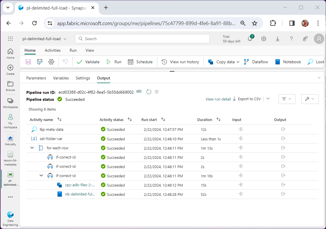
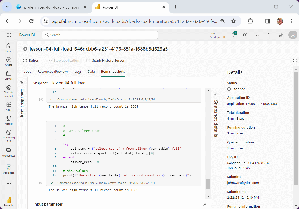
If will click on the output of the Spark Notebook, we get a link to the notebook snapshot.
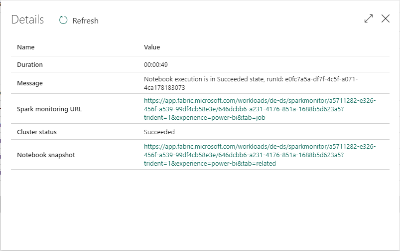
This snapshot was taken from the high temperature execution. We can tell by the debugging statements and record counts.
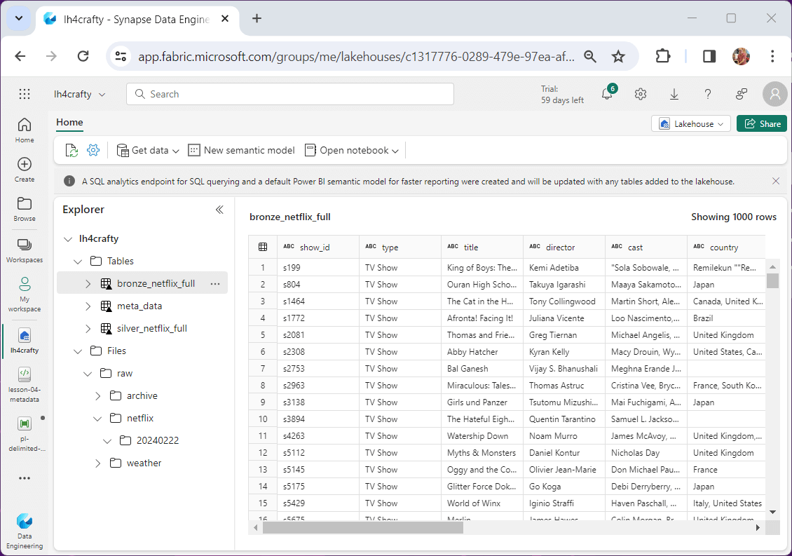
At the end of the first execution, we created a bronze and silver table for the Netflix titles. The image below shows a grid with the data.
At this time, please repeat the execution for each source. This can be done by incrementing the pipeline id and executing the pipeline.
While creating a meta data driven design takes some time, it is well worth the investment. Now, I can load hundreds of files into the lake by adding meta data to the table and scheduling the pipeline with the correct id.
Summary
Overall, I really do like the one stop shop idea of Fabric. Every you need is in one place with the Microsoft Fabric Service. Like any development team, Microsoft had to push the product out the door with a few rough edges.
The image below shows the three items that might have larger customers wait on adoption.
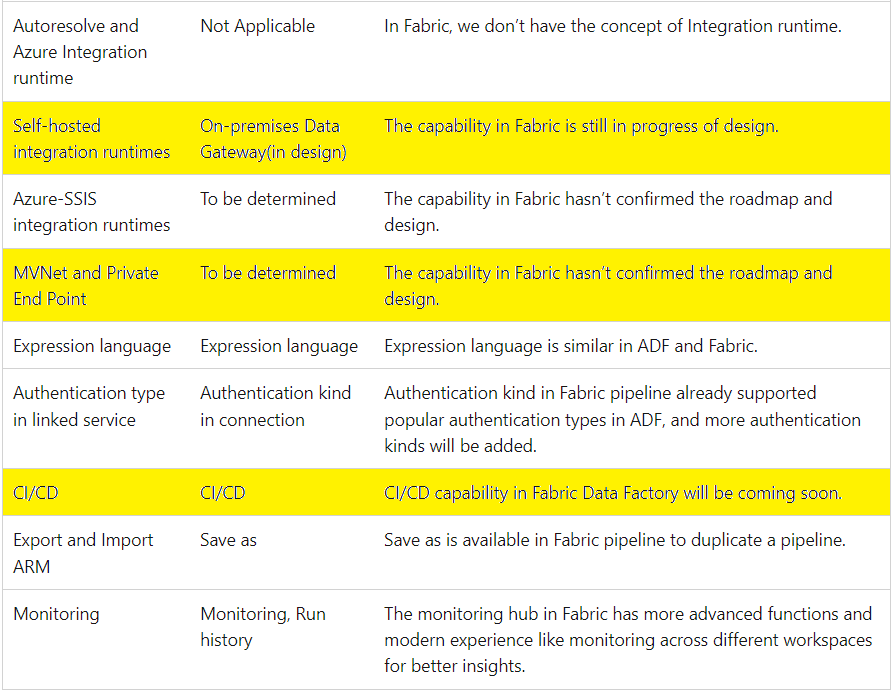
First, many companies still have a good percentage of their data on premises. Without a data gateway, older technologies such as SSIS will have to be used to land the data into a storage container.
Second, some companies like hospitals and financial institutions regard their data as highly sanative. The use of a virtual private network and endpoints has secured Azure components in the past. This support is not available in Fabric today.
Third, most companies have at least two environments: Development and Production. How do you move code from one environment to another? How do you keep track of versions? Spark Notebooks are easy since you can just download and upload files and manually check the code into git.
Data Factory is more complicated. It always has been a JSON export file that had many inter-dependencies. Some of the ADF complexity has gone away. A linked service and dataset are now replaced by a connection which is part of the data pipeline in fabric. Therefore, it might be possible to download and upload pipelines in the future? For now, we can move code by creating a pipeline with the same name as the demo – pl-delimited-full-load. Then hit the {} button to modify the JSON with the supplied definition in the zip file.
In short, the data gateway, private end points, and continuous integration / continuous deployment features are required to make this product shine. Enclosed is the zip file with the CSV data files, Data Pipeline in JSON format and Spark notebooks.