Data Presentation Layer

Microsoft Fabric allows the developer to create delta tables in the lake house. The bronze tables contain multiple versions of the truth, and the silver tables are a single version of the truth. How can we combine the silver tables into a model for consumption from the gold layer?

Business Problem

Our manager at Adventure Works has asked us to use a metadata-driven solution to ingest CSV files from external storage into Microsoft Fabric. A typical medallion architecture will be used in the design. The final goal of the project is to have end users access the gold layer tables using their favorite SQL tool.

Technical Solution

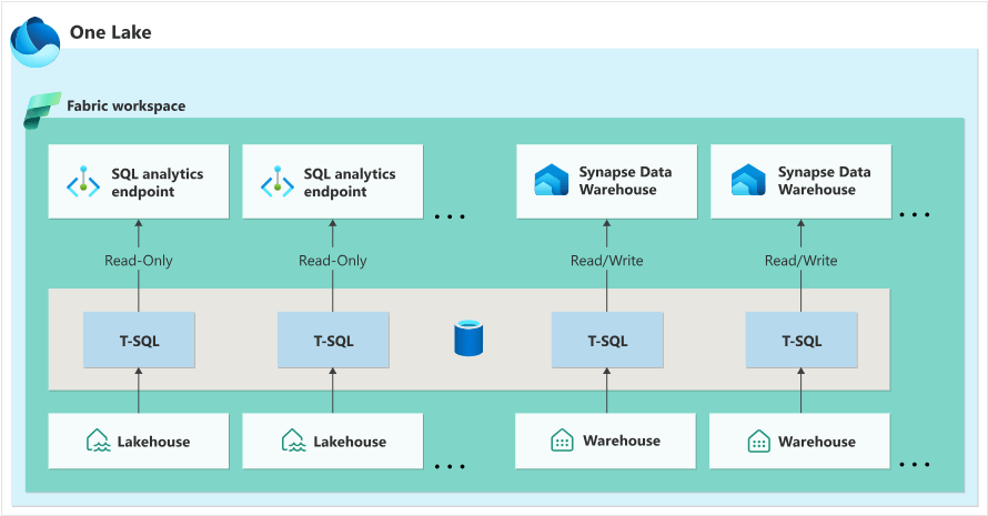
Microsoft Fabric supports two data warehouse components: SQL Analytics Endpoint and Synapse Data Warehouse. The image below shows that the endpoint is read-only while the warehouse supports both read and write operations. It makes sense to use the SQL Analytics Endpoint since we do not have to write to the tables.

The following topics will be covered in this article (thread).

1. create new lake house
2. create + populate metadata table
3. import + update child pipeline
4. create + execute parent pipeline
5. review bronze + silver tables
6. use warehouse view to combine tables
7. use warehouse view to aggregate table
8. connect to warehouse via SSMS

Architectural Overview

The architectural diagram for the metadata driven design is shown below. This is the child pipeline that I have been talking about. Please remember that the data pipeline uses a full refresh pattern. The bronze tables will contain all processed files and the silver tables will contained the most recent file (data).

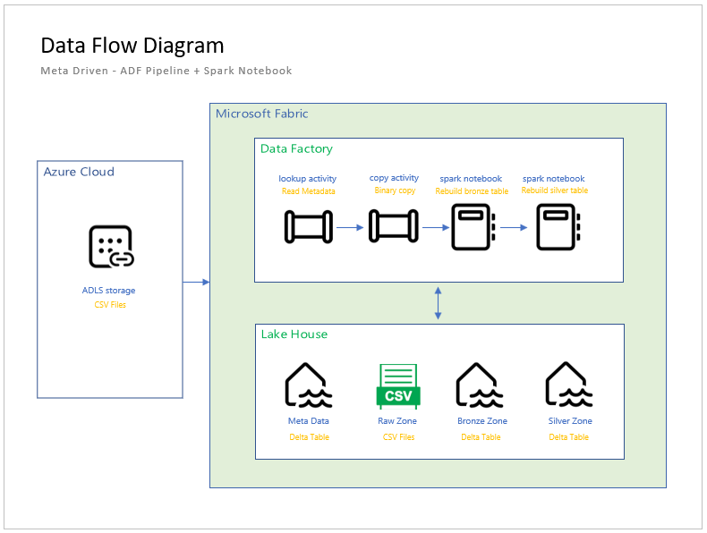
The parent pipeline will call the child pipeline for each meta data entry. At the end of a successful execution, the lake house has been created for all saleslt tables for both the bronze and silver zones. We will be working on the creating parent pipeline in this article.

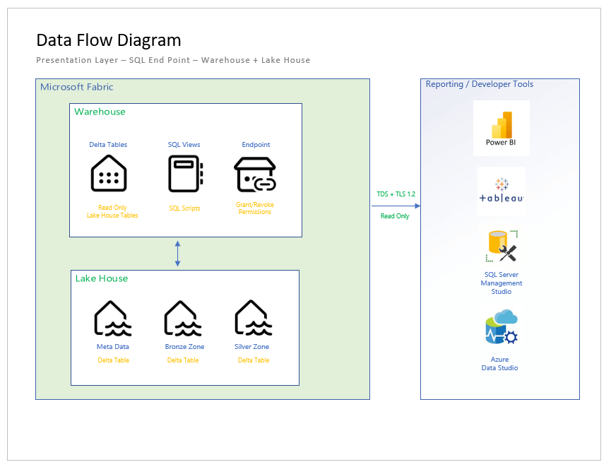
The above diagram shows how the presentation layer works. By default, all tables in the lake house (spark engine) are available to the SQL Analytics Endpoint as read only. To date, spark views are not supported. Do not fret. We can combine and aggregate data using SQL views in the data warehouse. After completing the warehouse or gold layer, we will retrieve data using my favorite tool (SQL Server Management Studio).

Meta Data Tables

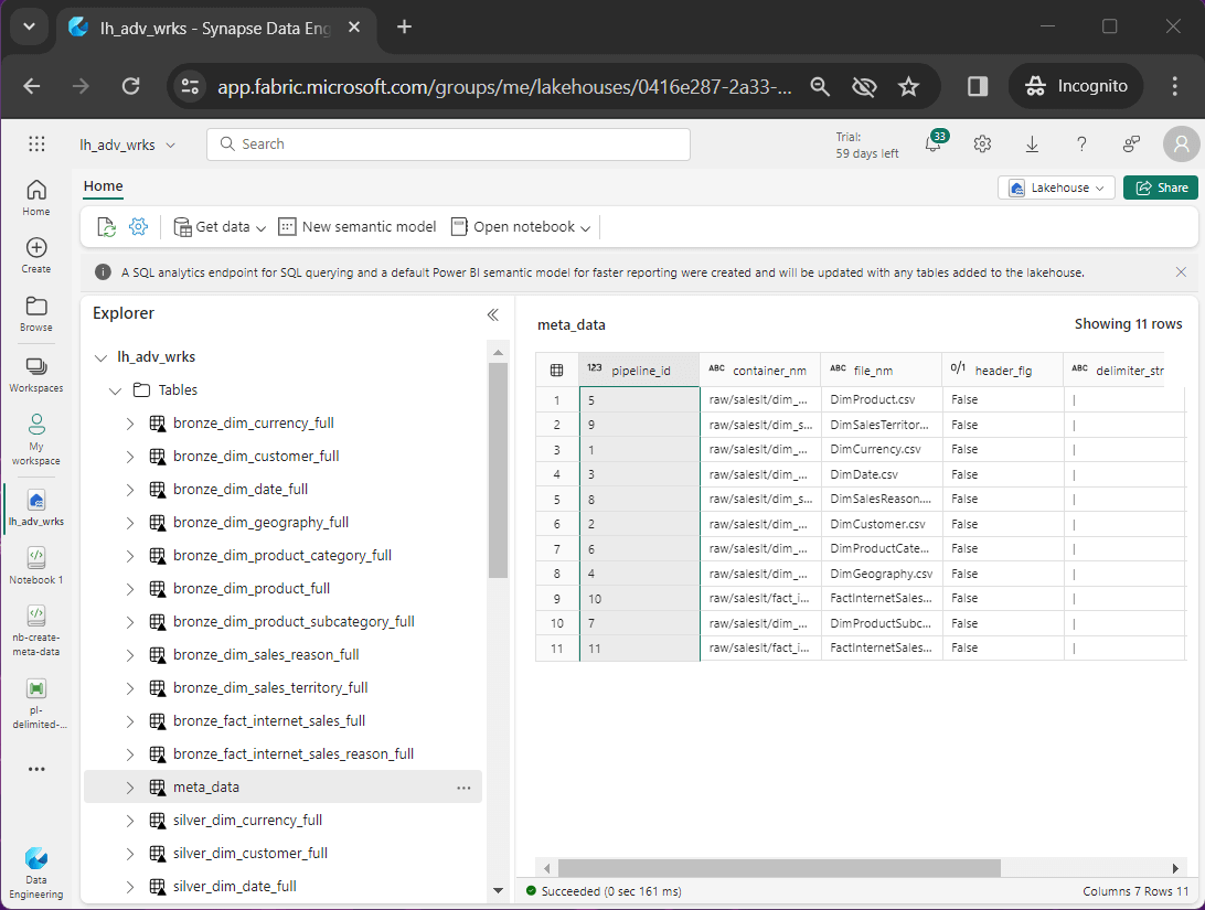
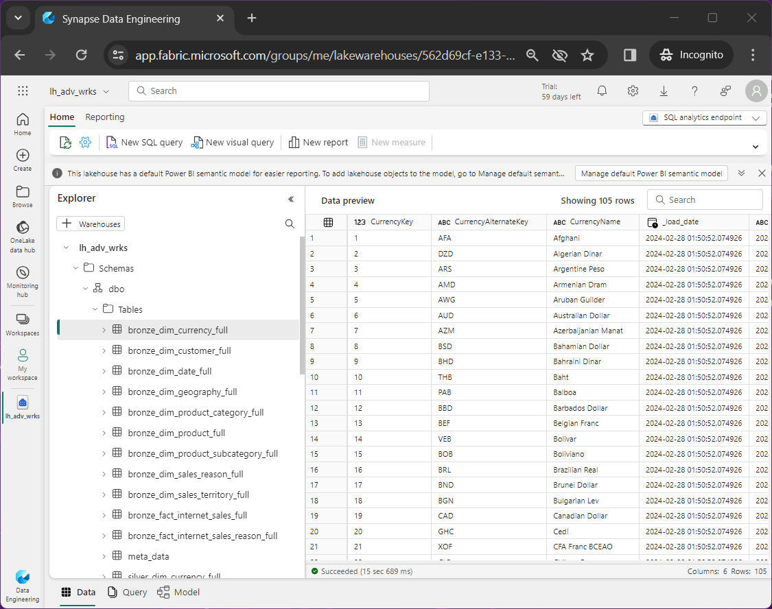
A meta data driven design allows the developer to automate the copying of data into the lake (raw files) as well as building the bronze and silver tables. The image below shows the meta data table viewed from the Lake House explorer. Please note, only the meta data table exists currently, and the local raw folder is empty.

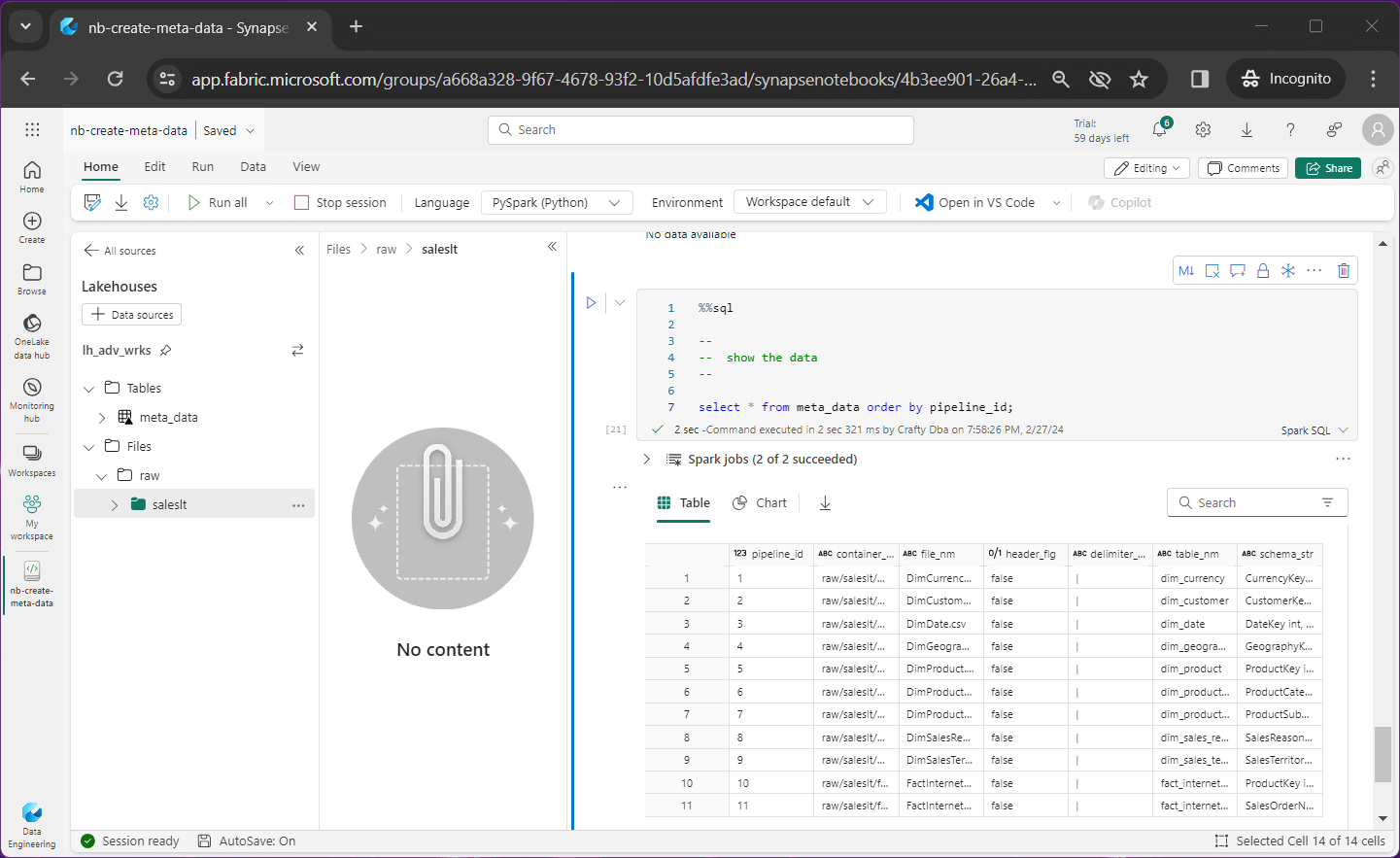
Let us review the meta data table right now with the following fields.

1. pipeline id – just an identifier
2. container name – same path in source and destination storage
3. file name – same file in source and destination storage
4. header flag – does the data file have a header line
5. delimiter string – how is the tuple divided into columns
6. table name – the root name of the table
7. schema string – infer schema or use this definition

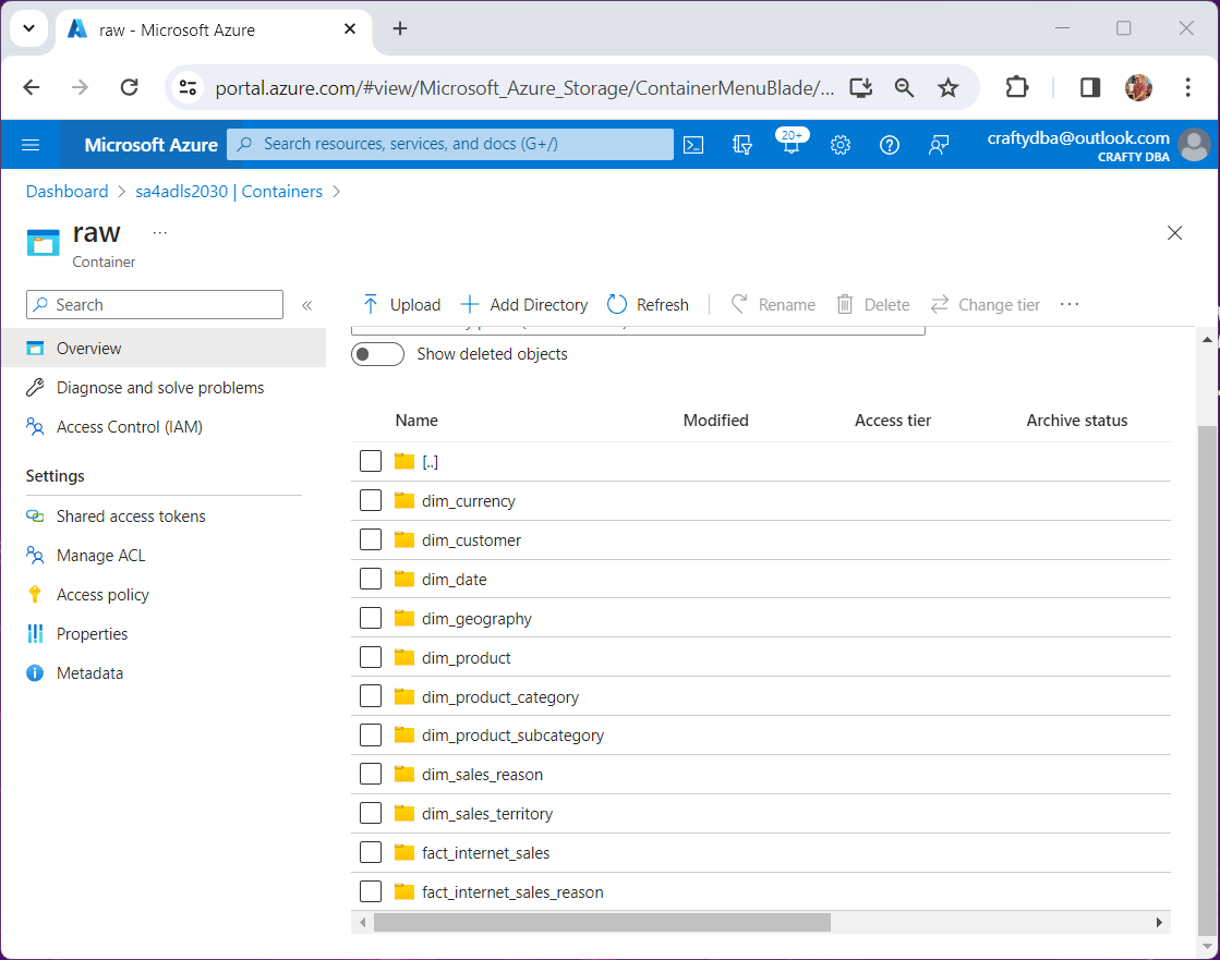
Each piece of information in the delta table is used by either the pipeline activities or spark notebooks to dictate which action to perform. Of course, there is a one-to-one mapping from source data files to rows of data in the meta data table. Please see the folder listing of the source storage account as shown below.

Please look at the nb-create-meta-data notebook for more details on how to reload the meta data table from scratch. Just download the zip file at the end of the article and find the file under the code folder.

Parent Pipeline

If you did not notice, I created a new lake house, named lh_adv_wrks. Since this task is so easy, I did not include any instructions. See the MS Learn webpage for more details.

The data pipeline, named pl-refresh-advwrks, is the parent pipeline we are building out today. It calls the child pipeline, named pl-delimited-full-load, with the pipeline id ranging from 1 to 11.

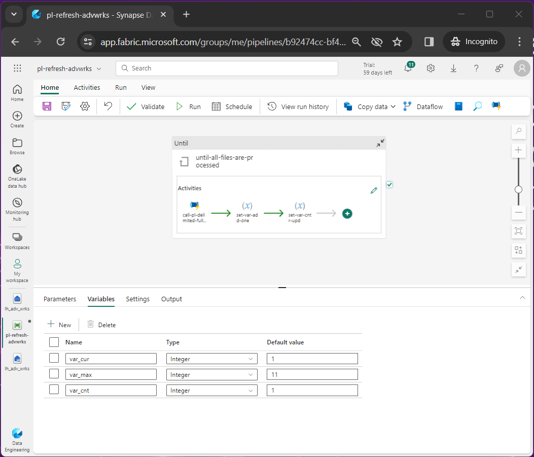
To write a while loop, we usually need two variables in a programming language like Python. The first variable is a counter and the second is the dynamic limit.

#
#  while loop - uses 2 variables
#

cnt = 1
lmt = 5
while cnt < lmt:
  print(f"Number is {cnt}!")
  cnt = cnt + 1

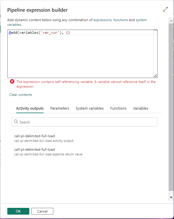
Data Factory does not allowed the developer to set a variable to itself. It is just a limitation of tool. The image below shows the error when trying to set the variable, named var_cnt, to itself plus one. The solution to this problem is to use another variable.

The image below shows the test condition for the until loop.

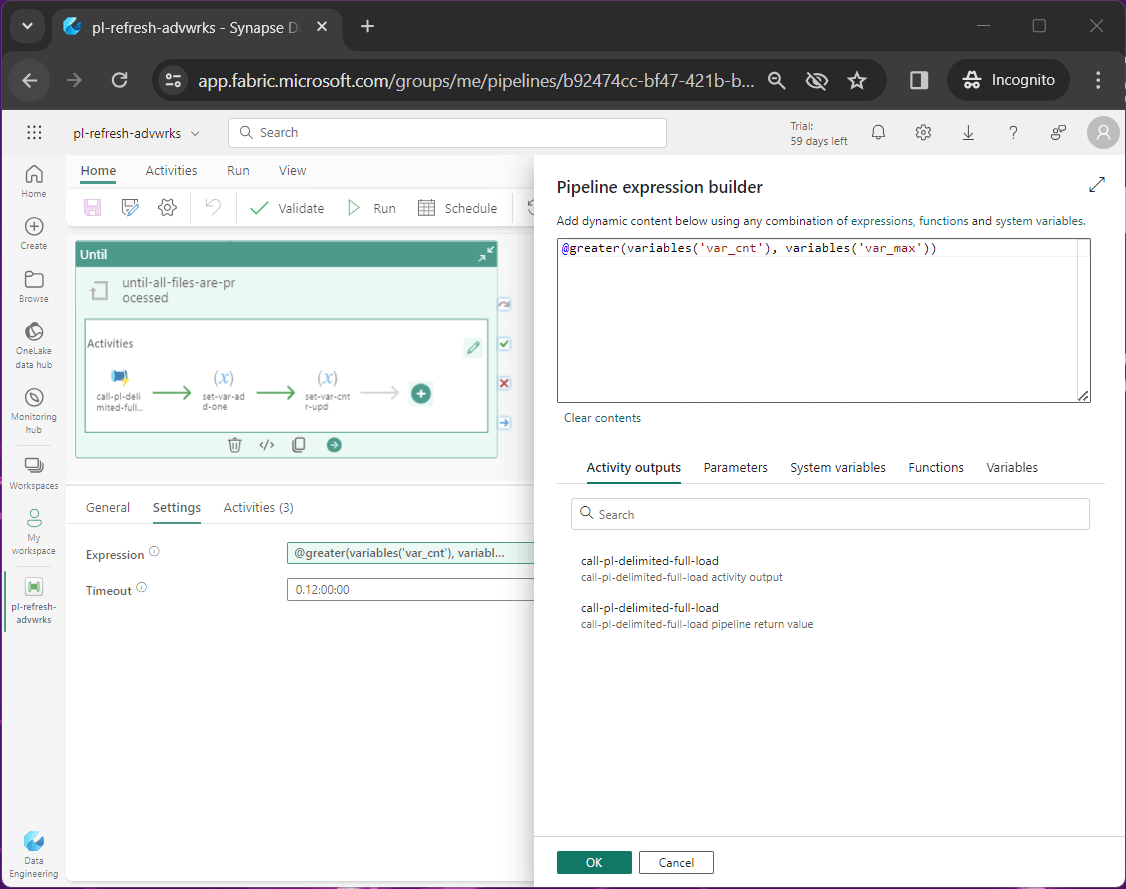
The variable, named var_cur, is used as a temporary variable since we cannot use self-assignment. Thus, we set the current value equal to the counter plus one.

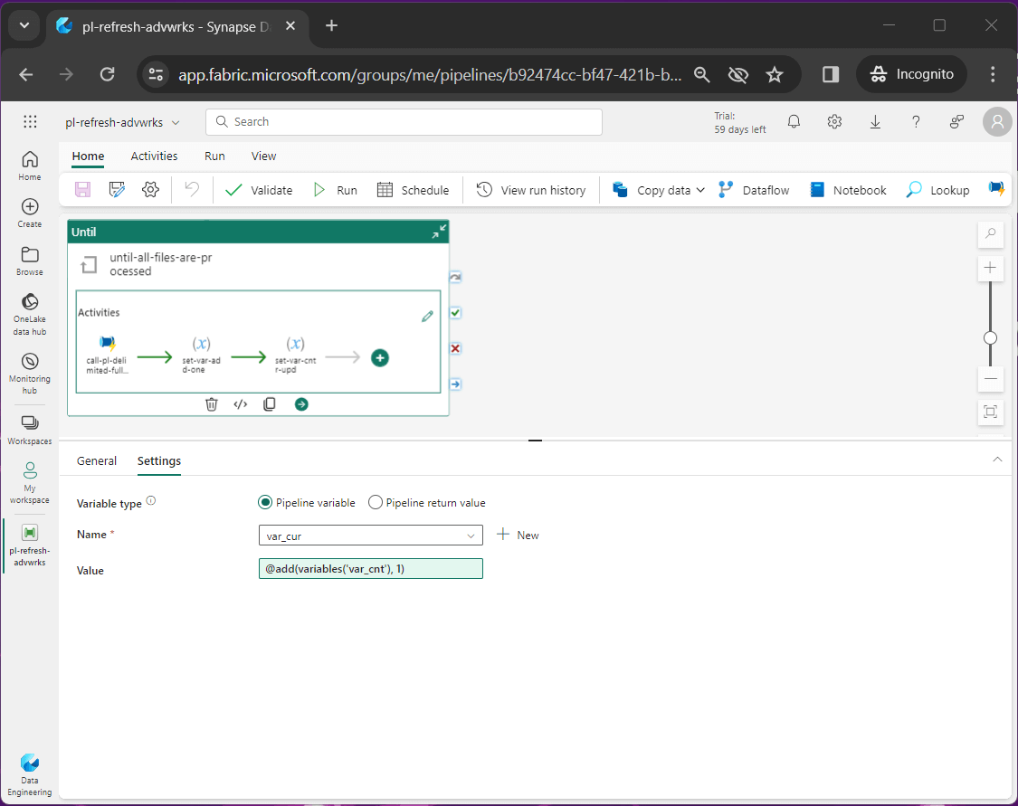
The last step of the process is to set the counter to the current value. See the assignment of the var_cnt variable below.

After successful execution of the parent pipeline, the lake house will contain refreshed data.

System Review

My workspace is where all the personal objects in Microsoft Fabric are listed.

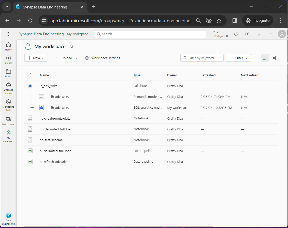
The table below shows the objects that are part of the Adventure Works lake house solution.

1. nb-create-meta-data – this delta table describes how to load the system
2. nb-delimited-full-load – read raw files, refresh bronze + silver tables
3. nb-test-schema – this Spark SQL code tests the schema used in meta data table
4. pl-delimited-full-load – copy file from source to raw, execute spark notebook
5. pl-refresh-advwrks – call the full load pipeline for all source files/li>
6. lh_adv_wrks – the lake house
   • SQL analytics endpoint – external programs can interact with lake via TDS
   • semantic model – the default Power BI data model

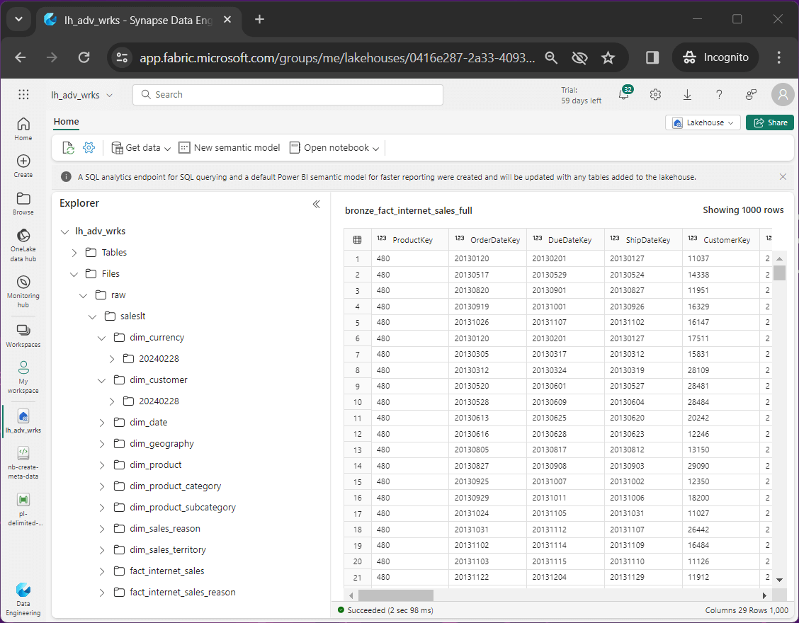
The One Lake is where all the action happens. If we right click on the lake house object and select open, the lake house explorer will be shown. The image below shows the versioning of data files in the raw zone for the adventure works dataset. Each time we execute the pipeline, a CSV file is copied to a sub-folder that has today’s date in sortable format.

The image below shows a bronze and silver table for each of the source files. There are a total of twenty-three delta tables shown by the explorer.

In the next section, we will be using the SQL analytics endpoint to create views for our presentation layer.

Data Warehouse

Make sure the key word warehouses is at the top of the explorer. In the lake house explorer, we have only tables and files. In the warehouse explorer, we can create other objects such as views, functions, and stored procedures. Today, we are focusing on views for our presentation layer.

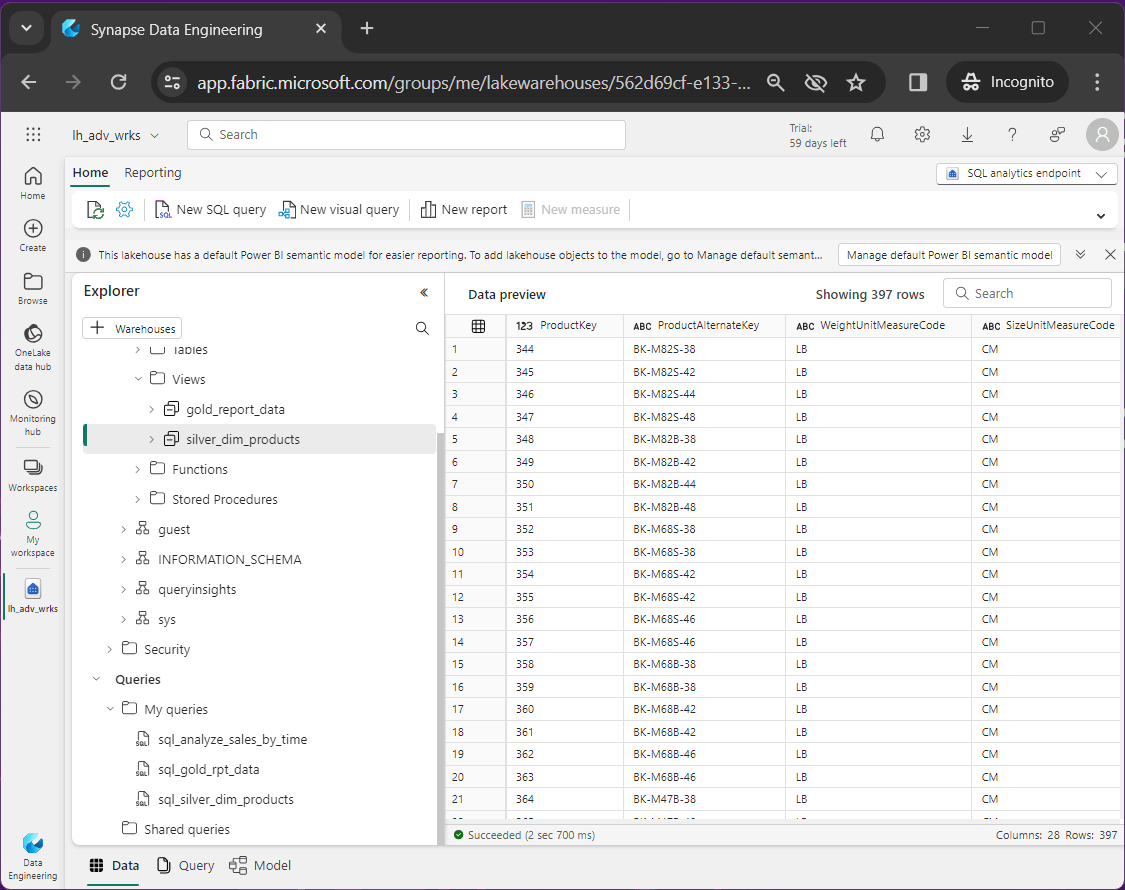
The first view we are going to create is named silver_dim_products. The SQL code below creates the view that combines the three product related tables into one dataset. It is a coin toss on what prefix to use on the table. I chose to use silver since we did not perform any calculations.

-- ******************************************************
-- *
-- * Name:         sql_silver_dim_products.txt
-- *
-- * Design Phase:
-- *     Author:   John Miner
-- *     Date:     03-01-2024
-- *     Purpose:  Combine 3 tables into one view.
-- *
-- ******************************************************
CREATE VIEW [silver_dim_products]
AS
SELECT
  p.ProductKey,
  p.ProductAlternateKey,
  p.WeightUnitMeasureCode,
  p.SizeUnitMeasureCode,
  p.EnglishProductName,
  p.StandardCost,
  p.FinishedGoodsFlag,
  p.Color,
  p.SafetyStockLevel,
  p.ReorderPoint,
  p.ListPrice,
  p.Size,
  p.SizeRange,
  p.Weight,
  p.DaysToManufacture,
  p.ProductLine,
  p.DealerPrice,
  p.Class,
  p.Style,
  p.ModelName,
  p.StartDate,
  p.EndDate,
  p.Status,
  sc.ProductSubcategoryKey,
  sc.ProductSubcategoryAlternateKey,
  sc.EnglishProductSubcategoryName,
  pc.ProductCategoryKey,
  pc.EnglishProductCategoryName
FROM
  silver_dim_product_full as p
JOIN
  silver_dim_product_subcategory_full as sc
ON
  p.ProductSubcategoryKey = sc.ProductSubcategoryKey
JOIN
  silver_dim_product_category_full as pc
ON
  pc.ProductCategoryKey = sc.ProductCategoryKey;

The output from previewing the SQL View is show below.

The view, named gold_report_data, combines data from six tables into one flattened dataset ready for reporting. See the code below for details. This table is truly a gold layer object.

-- ******************************************************
-- *
-- * Name:         sql_gold_report_data.txt
-- *
-- * Design Phase:
-- *     Author:   John Miner
-- *     Date:     03-01-2024
-- *     Purpose:  Combine tables for reporting.
-- *
-- ******************************************************
CREATE VIEW gold_report_data
AS
SELECT
  p.EnglishProductCategoryName
  ,Coalesce(p.ModelName, p.EnglishProductName) AS Model
  ,c.CustomerKey
  ,s.SalesTerritoryGroup AS Region
  , ABS(CAST((datediff(d, getdate(), c.BirthDate) / 365.25)AS INT)) as Age
  ,CASE
    WHEN c.YearlyIncome < 40000 THEN 'Low'
    WHEN c.YearlyIncome > 60000 THEN 'High'
    ELSE 'Moderate'
  END AS IncomeGroup
  ,d.CalendarYear
  ,d.FiscalYear
  ,d.MonthNumberOfYear AS Month
  ,f.SalesOrderNumber AS OrderNumber
  ,f.SalesOrderLineNumber AS LineNumber
  ,f.OrderQuantity AS Quantity
  ,f.ExtendedAmount AS Amount
FROM
  silver_fact_internet_sales_full as f
INNER JOIN
  silver_dim_date_full as d
ON
  f.OrderDateKey = d.DateKey
INNER JOIN
  silver_dim_products as p
ON
  f.ProductKey = p.ProductKey
INNER JOIN
  silver_dim_customer_full as c
ON
  f.CustomerKey = c.CustomerKey
INNER JOIN
  silver_dim_geography_full as g
ON
  c.GeographyKey = g.GeographyKey
INNER JOIN
  silver_dim_sales_territory_full as s
ON
  g.SalesTerritoryKey = s.SalesTerritoryKey;

The image below shows sample data from the table.

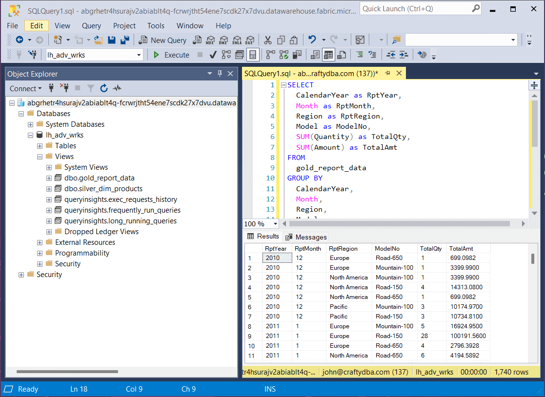
The last step is to use this flattened data in the gold view to figure out what sold best in December 2010 in North America. The bike model named “Road-150” was the top seller.

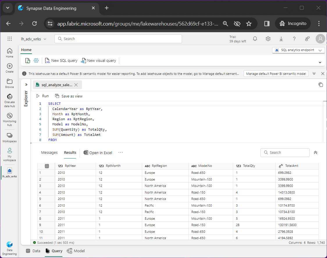
The SQL query seen below was used to generate the previous result set.

-- ******************************************************
-- *
-- * Name:         sql_analyze_sales_by_time.txt
-- *
-- * Design Phase:
-- *     Author:   John Miner
-- *     Date:     03-01-2024
-- *     Purpose:  Combine tables for reporting.
-- *
-- ******************************************************
SELECT
  CalendarYear as RptYear,
  Month as RptMonth,
  Region as RptRegion,
  Model as ModelNo,
  SUM(Quantity) as TotalQty,
  SUM(Amount) as TotalAmt
FROM
  gold_report_data
GROUP BY
  CalendarYear,
  Month,
  Region,
  Model
ORDER BY
  CalendarYear,
  Month,
  Region;

What I did not cover is the fact that any SQL scripts that are created by hand or by right click are stored in the section called My Queries. These queries can be pulled up and re-executed any time you want. Just like a SQL database, an object must be dropped before being created again.

Using the SQL endpoint

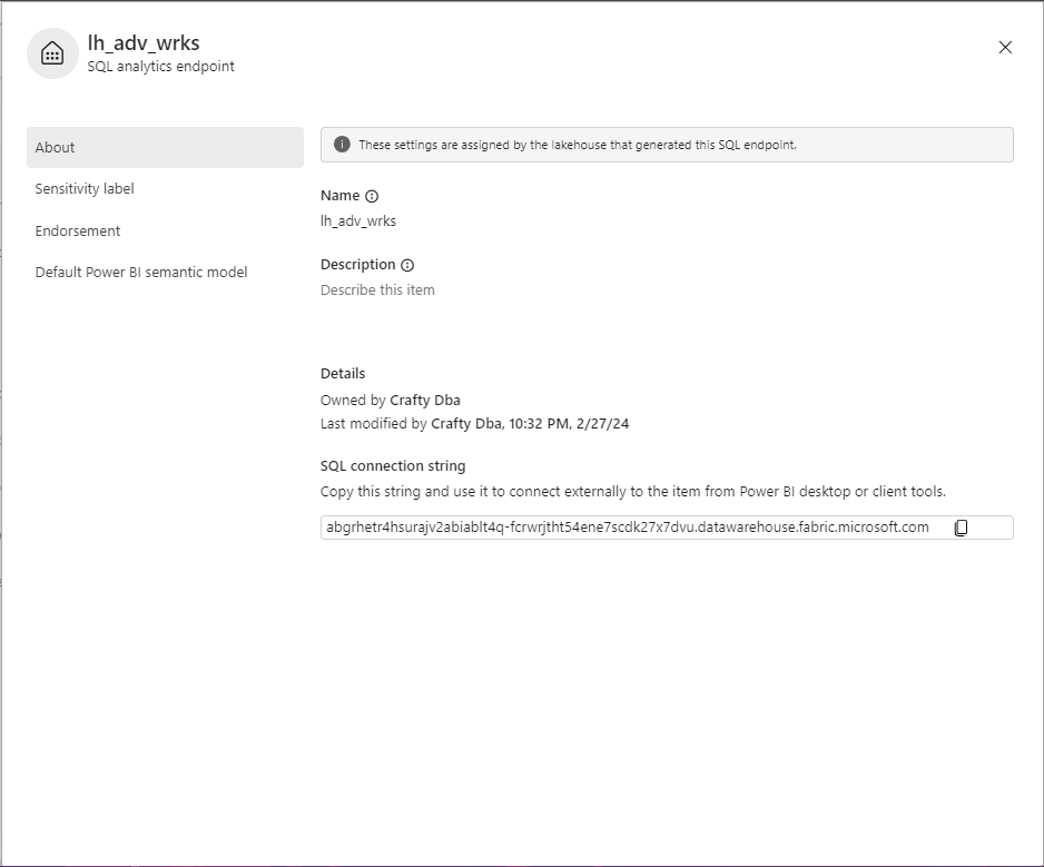
We need to retrieve the fully qualified name of the SQL analytics endpoint. Use the copy icon to retrieve this long string.

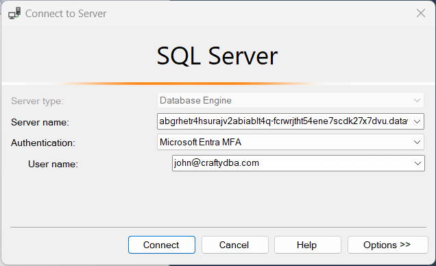
Fabric only supports Microsoft Entra, formally known as Azure Active Directory with multi-factory authentication (MFA). The image below shows the most recent SQL Server Management Studio making a connection to the SQL endpoint. The user named john@craftydba.com is signing into the service.

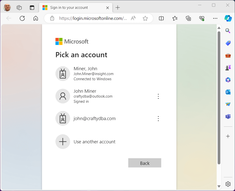
The login action from SSMS will open a web browser to allow the end user to enter credentials. Since I work with many different accounts, I must choose the correct username.

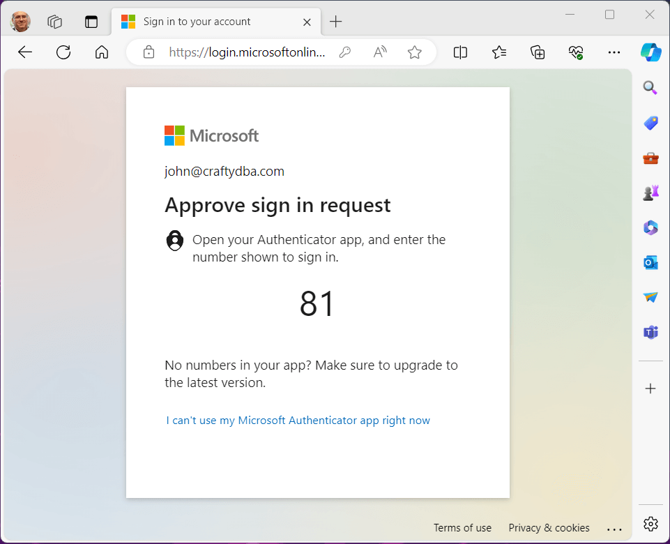
The authenticator application is used to verify that the correct user is signing into the system.

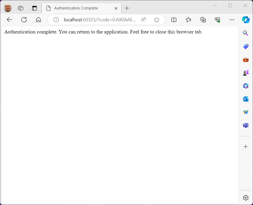
Once authentication is complete, we can close the web browser window.

The last step is to make sure the result set that was created in our Fabric Data Warehouse matches the result set retrieved by SSMS using the SQL end point.

The real power of the One Lake is the ability to mesh data sets from a variety of locations into one place. The SQL analytics end point allows users to leverage existing reports and/or developer tools to look at the data in the warehouse.

Summary

One thing I really like about Microsoft Fabric is the fact that all the services are in one place. Today, we covered the parent/child pipeline design. The parent pipeline retrieves the list of meta data from the delta table. For each row, data is copied from the source location to the raw layer. Additionally, a bronze table showing history is created as well as a silver table showing the most recent data. This is a full refresh load pattern with history for auditing.

Once the data is in the lake house, we can use the data warehouse section of Fabric to create views that combine tables, aggregate rows and calculate values. This data engineering is used to clean the data for reporting or machine learning.

Finally, there are two ways to use the data. The semantic model is used by Power BI reports that a built into Fabric. The SQL analytics endpoint is used for external reporting and/or developer tools to access the data. The steps to access the warehouse are pretty like any relational database management system that we might access.

Next time, I will be talking about how end users can update files in the Lakehouse using the one lake explorer. Enclosed is the zip file with the CSV data files, Data Pipelines in JSON format, Spark notebooks and SQL notebooks.