Introduction

The SSIS Data Flow is a high-speed asynchronous data pipeline. In this article I discuss some of what’s happening "under the hood" of a Data Flow Task.

To build the demo project described in this article you will need SSIS 2005 and the AdventureWorks sample database (which can be downloaded at http://www.codeplex.com/MSFTDBProdSamples/Release/ProjectReleases.aspx?ReleaseId=4004).

Create and Configure a Source

Start by creating a new SSIS project. I named my project DataFlowProbe. Drag a Data Flow Task onto the Control Flow and double-click it to open the Data Flow edit tab.

Drag an OLE DB Source onto the Data Flow canvas and double-click it to open the editor. Click the New button beside the OLE DB Connection Manager dropdown:

If you have configured a connection to AdventureWorks before, select it from the Data Connections list. If not, click the New button. Enter a server name and select AdventureWorks for the Database name:

Click OK until you return to the OLE DB Source Adapter. Change the Data Access Mode to SQL Command and paste the following command into the SQL Command Text textbox:

Select
  ContactID
 ,Title
 ,FirstName
 ,MiddleName
 ,LastName
 ,EmailAddress
 ,Phone
FromPerson.Contact

Click OK to close the OLE DB Source Adapter editor.

Create and Configure a Destination

Drag an OLE DB Destination Adapter onto the data flow canvas and rename it ContactStage. Connect a data flow pipeline from the OLE DB Source to ContactStage and double-click ContactStage to open the editor. Accept the defaults (the Connection Manager will be set to AdventureWorks and the data access mode will be set to “Table or view – fast load”). Click the New button beside the “Name of the table or the view” dropdown.

Something amazing happens: The Create Table dialog opens containing T-SQL to create a new table:

CREATETABLE [ContactStage] (
    [ContactID] INTEGER,
    [Title] NVARCHAR(8),
    [FirstName] NVARCHAR(50),
    [MiddleName] NVARCHAR(50),
    [LastName] NVARCHAR(50),
    [EmailAddress] NVARCHAR(50),
    [Phone] NVARCHAR(25)
)

The new table is named ContactStage. SSIS got that name from the name of the OLE DB Destination Adapter. The columns Data Definition Language (DDL) was generated from the data flow path. We’ll look at this in a bit.

Click OK to create the table (it’s actually created once you click the OK button on the Create Table dialog). Click the Mappings page to complete the configuration of the ContactStage OLE DB Destination Adapter. Auto-mapping occurs between columns with the same name and data type. Since the destination was created from the definition of the incoming rows, they all have the same name and data type; so they all auto-map:

Click OK to close the editor.

Now you may think I’m crazy, but this is how I actually develop SSIS packages. It’s fast and works for me – and works well, in fact.

What’s in the Path?

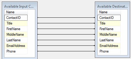
Right-click the data flow path connecting and click Edit. Click the Metadata page to view the columns defined in the data flow path:

This is a peek under the hood of the Data Flow Task. This was used to generate the DDL in the Create Table T-SQL we observed in the ContactStage OLE DB Destination. I haven’t written T-SQL to create a staging table for SSIS since 2005.

A Bit of Simulation

To simulate some data flow transformations, drag a couple Union All transformations onto the Data Flow canvas. Connect the Union All transformations between the Source and Destination adapters as shown:

This now simulates some transformations inside the Data Flow.

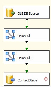
What’s wrong with the Destination?

Caught that, did you? There’s a red circle with a white X inside the ContactStage OLE DB Destination Adapter. Hovering over it reveals the issue is:

input column "ContactID" (130) has lineage ID 32 that was not previously used in the Data Flow task.

So what happened? The short version is I broke the data flow when I added the Union All transformations.

Transformations have input and output buffers. One way to look at buffers is as interfaces between Data Flow components. Output buffers connect to input buffers, and this is how data is routed through the data flow pipeline.

Buffers contain a column collection which contains columns (remember the Data Flow Path metadata page?). Rows flow into the input buffer, are acted upon in the transformation, and flow out of the output buffer. Some transformations reuse buffers; others copy buffers from the input to output. If buffers are reused the transformation is synchronous. If buffers are copied the transformation is asynchronous.

The column definitions inside the buffers are visible in the Data Flow Path metadata. One thing the metadata page doesn’t show us is the Lineage ID property of the column. It’s an integer and it’s unique throughout the data flow. When buffers are reused, the Lineage ID doesn’t change – it’s the same column at the input and output. When buffers are copied, a new column is created – which gets a new (unique) Lineage ID.

Union All transformations copy buffers. The validation (unfortunately) checks one column at a time. It has found the first column – named ContactID – used to have a Lineage ID of 32. The full extent of the damage I did by inserting a buffer-copying transformation into the flow is evident when I double-click the ContactStage Destination in an attempt to open the editor:

This scenario occurs with enough frequency to justify the Restore Invalid Column References Editor, shown above. The ContactID column with Lineage ID 32 is shown as invalid, but the References Editor located (and suggests) a column with the same name and data type: the ContactID column with Lineage ID 333. In fact, it’s located new columns for all the invalid references (although the error did not report these additional columns).

Click OK to replace the invalid references with the suggested columns.

Observing the Haystack

If you run the project in debug mode as it’s now built, you will see a couple / three buffers of data flow through. You can examine each row flowing between the Union All transformations by adding a Data Viewer. Right-click the Data Flow Path connecting Union All to Union All 1, then click Data Viewers.

Click the Add button when the Data Flow Path Editor displays. When the Configure Data Viewer displays, accept the default Grid type and click OK:

Click OK to close the Data Flow Path Editor. The Data Flow Path now displays an icon to indicate a data viewer is present on the Data Flow Path:

When you execute the package in debug mode, a data viewer displays showing all the contents of the buffer:

The data viewer acts as a breakpoint in the Data Flow – pausing execution while you view the data in one buffer. If you close the data viewer, the data continues to flow as if there were no data viewer. If you click the green “play” button in the upper left, the data viewer releases the current buffer and pauses on the next buffer flowing through the Data Flow Path. Clicking the Detach button allows all data to flow until completion or until you again click the same button (the text on the button changes to “Attach” when you click the Detach button).

Finding the Needle

This is all well and good if you have a few hundred – or even a few thousand – rows flowing through your data flow. It can take a while to wait for row 6,578,361 of 10,000,000 rows to show up. So how do you find the needle in the haystack?

I like to use a design pattern I call a Data Probe.

To construct a data probe, add two Multicast transformations and a Conditional Split transformation to the Data Flow. Connect one Multicast between the Union All transformations. This will allow the current data flow to continue uninterrupted.

Connect a second output from the Multicast to the Conditional Split transformation. Leave the output of the Conditional Split transformation disconnected for now:

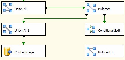
The second output of the first Multicast will send the same rows to the Conditional Split transformation as are sent to the Union All 1 transformation.

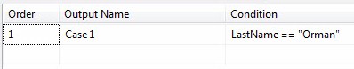
Double-click the Conditional Split to open the editor. Add the following expression to the top row:

LastName == "Orman"

Connect the output of the Conditional Split transformation to the second Multicast transformation (the second Multicast is merely an endpoint for the output of the Conditional Split transformation). When prompted, select the Case 1 output to connect to the Multicast input:

Create a grid data viewer on the data flow path between the Conditional Split and second Multicast transformations:

Execute the package in debug mode. Note the only row present at the “Case 1” output of the Conditional Split transformation is the needle for which you were searching in the haystack.

Conclusion

There are other ways to isolate rows in a data flow. Data probes are helpful and take a couple minutes to construct.