In my previous article, “SSIS Basics: Setting Up Your Initial Package“, I showed you how to create an SSIS package and configure connection managers, data sources, and data source views. In this article, I will show you how to use some of those data connections to retrieve data from a SQL Server database and load the data into an Excel file. I will also show you how to add a computed column based on data derived from the data flow. In addition, I will demonstrate how to run the package.

SSIS supports many control flow items that manage a package’s workflow, but the one I think to be the most important and most often used is the Data Flow task. For this reason, I focus on that task in this article. In future articles, I’ll cover other control flow items.

Adding a Data Flow Task

Our goal in creating this package is to move data from a SQL Server database to an Excel file. As part of that goal, we also want to insert an additional column into the Excel file that’s based on derived data.

To carry out our goal, we must add a Data Flow task to our control flow. The task lets us retrieve data from our data source, transform that data, and insert it into our destination, the Excel file. The Data Flow task is one of the most important and powerful components in SSIS and as such has it’s own workspace, which is represented by the Data Flow tab in SSIS Designer, as shown in Figure 1.

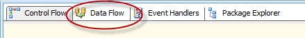
Figure 1: The Data Flow tab in SSIS Designer

Before we can do anything on the Data Flow tab, we must first add a Data Flow task to our control flow. To add the task, drag it from the Control Flow Items window to the Control Flow tab of the SSIS Designer screen, as illustrated in Figure 2.

Figure 2: Adding a Data Flow task to the control flow

To configure the data flow, double-click the Data Flow task in the control flow. This will move you to the Data Flow tab, shown in Figure 3.

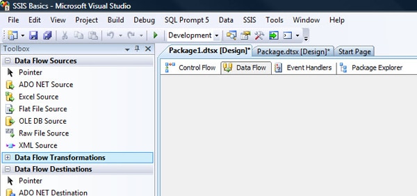
Figure 3: The Data Flow tab in SSIS Designer

Configuring the Data Flow

You configure a Data Flow task by adding components to the Data Flow tab. SSIS supports three types of data flow components:

• Sources: Where the data comes from
• Transformations: How you can modify the data
• Destinations: Where you want to put the data

A Data Flow task will always start with a source and will usually end with a destination, but not always. You can also add as many transformations as necessary to prepare the data for the destination. For example, you can use the Derived Column transformation to add a computed column to the data flow, or you can use a Conditional Split transformation to split data into different destinations based on specified criteria. This and other components will be explained in future articles.

To add components to the Data Flow task, you need to open the Toolbox if it’s not already open. To do this, point to the View menu and then click ToolBox, as shown in Figure 4.

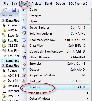
Figure 4: Opening the Toolbox to view the data flow components

At the left side of the Data Flow tab, you should now find the Toolbox window, which lists the various components you can add to your data flow. The Toolbox organizes the components according to their function, as shown in Figure 5.

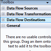
Figure 5: The component categories as they appear in the Toolbox

To view the actual components, you must expand the categories. For example, to view the source components, you must expand the Data Flow Sources category, as shown in Figure 6

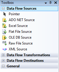
Figure 6: Viewing the data flow source components

Adding an OLE DB Source

The first component we’re going to add to the data flow is a source. Because we’re going to be retrieving data from a SQL Server database, we’ll use an OLE DB source. To add the component, expand the Data Flow Sources category in the Toolbox. Then drag an OLE DB source from to the Data Flow window. Your data flow should now look similar to Figure 7.

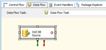
Figure 7: Adding an OLE DB source to your data flow

You will see that we have a new item named OLE DB Source. You can rename the component by right-clicking it and selecting rename. For this example, I renamed it Employees.

There are several other features about the OLE DB source noting:

• A database icon is associated with that source type. Other source types will show different icons.
• A reversed red X appears to the right of the name. This indicates that the component has not yet been properly configured.
• Two arrows extend below the component. These are called data paths. In this case, there is one green and one red. The green data path marks the flow of data that has no errors. The red data path redirects rows whose values are truncated or that generate an error. Together these data paths enable the developer to specifically control the flow of data, even if errors are present.

To configure the OLE DB source, right-click the component and then click Edit. The OLE DB Source Editor appears, as shown in Figure 8.

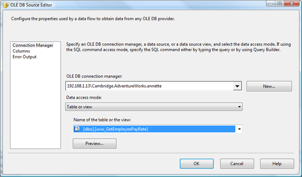
Figure 8: Configuring the OLEDB source

From the OLE DB connection manager drop-down list, select the OLE DB connection manager we set up in the last article, the one that connects to the AdventureWorks database.

Next, you must select one of the following four options from the Data access mode drop-down list:

• Table or view
• Table name or view name variable
• SQL command
• SQL command from variable

For this example, we’ll select the Table or View option because we’ll be retrieving our data through the uvw_GetEmployeePayRate view, which returns the latest employee pay raise and the amount of that raise. Listing 1 shows the Transact-SQL used to create the view in the AdventureWorks database.

Listing 1: The uvw_GetEmployeePayRate view definition

After you ensure that Table or view is selected in the Data access mode drop-down list, select the uvw_GetEmployeePayRate view from the Name of the table or the view drop-down list. Now go to the Columns page to select the columns that will be returned from the data source. By default, all columns are selected. Figure 9 shows the columns (EmployeeID, RateChangeDate, and Rate) that will be added to the data flow for our package, as they appear on the Columns page.

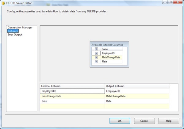
Figure 9: The Columns page of the OLE DB Source Editor

If there are columns you don’t wish to use, you can simply uncheck them in the Available External Columns box.

Now click on the Error Output page (shown in Figure 10) to view the actions that the SSIS package will take if it encounters errors.

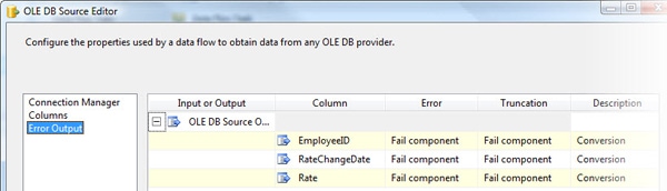
Figure 10: The Error Output page of the OLE DB Source Editor

By default, if there is an error or truncation, the component will fail. You can override the default behavior, but explaining how to do that is beyond the scope of this article. You’ll learn about error handling in future articles.

Now return to the Connection Manager page and click the Preview button to view a sample dataset in the Preview Query Results window, shown in Figure 11. Previewing the data ensures that what is being returned is what you are expecting.

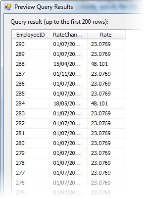
Figure 11: Previewing a sample dataset

After you’ve configured the OLE DB Source component, click OK.

Adding a Derived Column Transformation

The next step in configuring our data flow is to add a transformation component. In this case, we’ll add the Derived Column transformation to create a column that calculates the annual pay increase for each employee record we retrieve through the OLE DB source.

To add the component, expand the Data Flow Transformations category in the Toolbox window, and drag the Derived Column transformation (shown in Figure 12) to the Data Flow tab design surface.

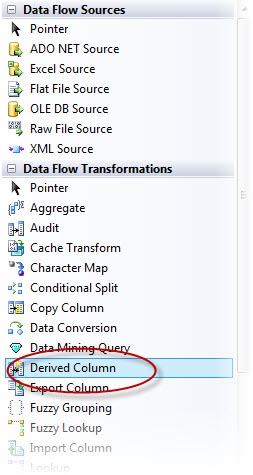
Figure 12: The Derived Column transformation as its listed in the Toolbox

Drag the green data path from the OLE DB source to the Derived Column transformation to associate the two components, as shown in Figure 13. (If you don’t connect the two components, they won’t be linked and, as a result, you won’t be able to edit the transformation.)

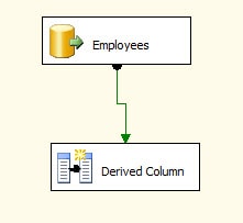
Figure 13: Using the data path to connect the two components

The next step is to configure the Derived Column component. Double-click the component to open the Derived Column Transformation Editor, as shown in Figure 14.

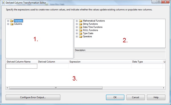
Figure 14: Configuring the Derived Column transformation

This editor is made up of three regions, which I’ve labeled 1, 2 and 3:

1. Objects you can use as a starting point. For example you can either select columns from your data flow or select a variable. (We will be working with variables in a future article.)
2. Functions and operators you can use in your derived column expression. For example, you can use a mathematical function to calculate data returned from a column or use a date/time function to extract the year from a selected date.
3. Workspace where you build one or more derived columns. Each row in the grid contains the details necessary to define a derived column.

For this exercise, we’ll be creating a derived column that calculates a pay raise for employees. The first step is to select the existing column that will be the basis for our new column.

To select the column, expand the Columns node, and drag the Rate column to the Expression column of the first row in the derived columns grid, as shown in Figure 15.

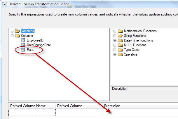
Figure 15: Adding a column to the Expression column of the derived column grid

When you add your column to the Expression column, SSIS prepopulates the other columns in that row of the grid, as shown in Figure 16.

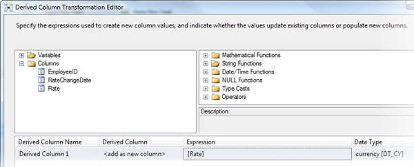
Figure 16: Prepopulated values in derived column grid

As you can see, SSIS has assigned our derived column the name Derived Column 1 and set the Derived Column value to <add as new column>. In addition, our [Rate] field now appears in the Expression column, and the currency[DT_CY] value has been assigned to the Data Type column.

You can change the Derived Column Name value by simply typing a new name in the box. For this example, I’ve renamed the column NewPayRate.

For the Derived Column value, you can choose to add a new column to your data flow (which is the default value, <add as new column>) or to replace one of the existing columns in your data flow. In this instance, we’ll add a new column, but there may be times when overwriting a column is required.

The data type is automatically created by the system and can’t be changed at this stage.

Our next step is to refine our expression. Currently, because only the Rate column is included in the expression, the derived column will return the existing values in that column. However, we want to calculate a new pay rate. The first step, then, is to add an operator. To view the list of available operators, expand the list and scroll through them. Some of the operators are for string functions and some for math functions.

To increase the employee’s pay rate by 5%, we’ll use the following calculation:

[Rate] * 1.05

To do this in the Expression box, either type the multiplication operator (*), or drag it from the list of operators to our expression (just after the column name), and then type 1.05, as shown in Figure 17.

Figure 17: Defining an expression for our derived column

You will see that the Data Type has now changed to numeric [DT_NUMERIC].

Once you are happy with the expression, click on OK to complete the process. You will be returned to the Data Flow tab. From here, you can rename the Derived Column transformation to clearly show what it does. Again, there are two data paths to use to link to further transformations or to connect to destinations.

Adding an Excel Destination

Now we need to add a destination to our data flow to enable us to export our results into an Excel spreadsheet.

To add the destination, expand the Data Flow Destinations category in the Toolbox, and drag the Excel destination to the SSIS Designer workspace, as shown in Figure 18.

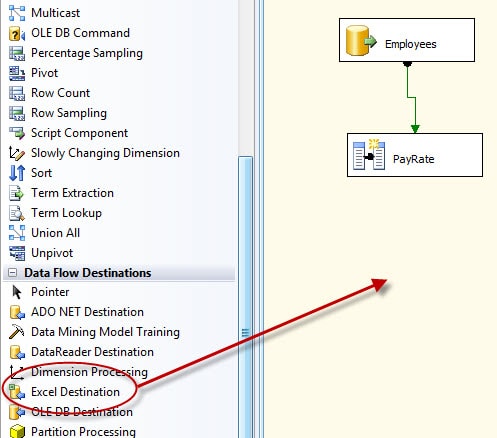
Figure 18: Adding an Excel destination to your data flow

Now connect the green data path from the Derived Column transformation to the Excel destination to associate the two components, as shown in Figure 19.

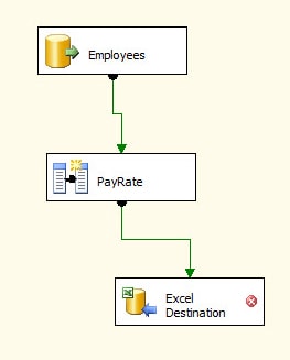
Figure 19: Connecting the data path from the transformation to the destination

As you can see, even though we have connected the PayRate transformation to the Excel destination, we still have the reversed red X showing us that there is a connection issue. This is because we have not yet selected the connection manager or linked the data flow columns to those in the Excel destination.

Next, right-click the Excel destination, and click Edit. This launches the Excel Destination Editor dialog box, shown in Figure 20. On the Connection Manager page, under OLE DB connection manager, click on the New button then under Excel File Path click on the Browse button and select the file you created in the previous article and click on OK, then under Name of the Excel Sheet select the appropriate sheet from the file.

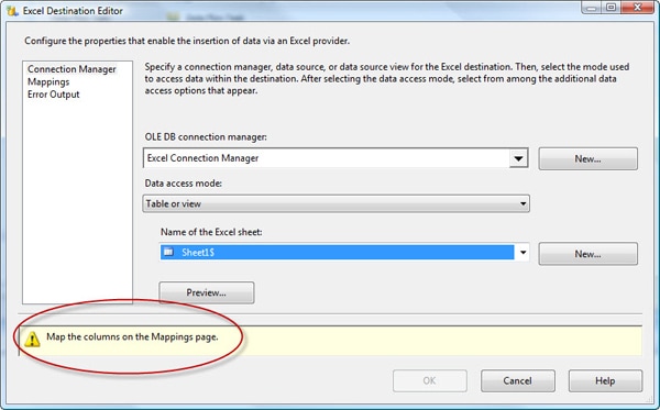
Figure 20: Configuring the Excel destination component

At the bottom of the Connection Manager page, you’ll notice a message that indicates we haven’t mapped the source columns with the destination columns. To do this, go to the Mappings page (shown in Figure 21) and ensure that the columns in the data flow (the input columns) map correctly to the columns in the destination Excel file. The package will make a best guess based on field names; however, for this example, I have purposefully named my columns in the excel spreadsheet differently from those in the source database so they wouldn’t be matched automatically.

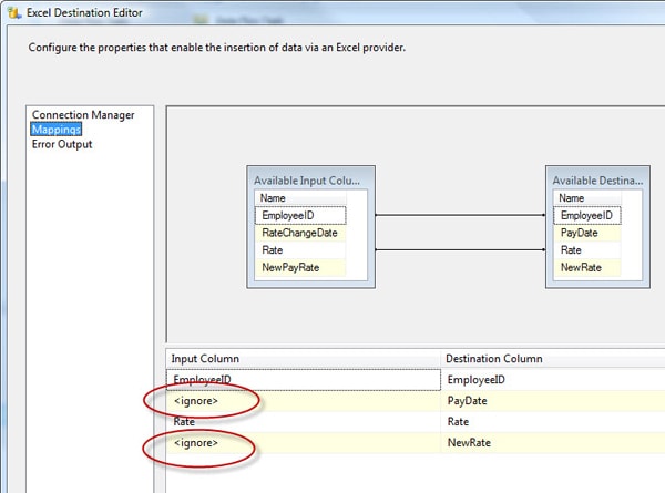
Figure 21: The Mappings page of the Excel Destination Editor

To match the remaining columns, click the column name in the Input Column grid at the bottom of the page, and select the correct column. As you select the column, the list will be reduced so that only those columns not linked are available. At the same time, the source and destination columns in the top diagram will be connected by arrows, as shown in Figure 22.

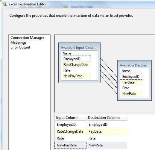
Figure 22: Mapping the columns between the data flow and the destination

Once you’ve properly mapped the columns, click OK. The Data Flow tab should now look similar to the screenshot in Figure 23.

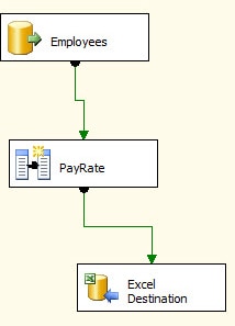
Figure 23: The configured data flow in your SSIS package

Running an SSIS Package in BIDS

Now all we need to do is execute the package and see if it works. To do this, click the Execute button. It’s the green arrow on the toolbar, as shown in Figure 24.

Figure 24: Clicking the Execute button to run your SSIS package

As the package progresses through the data flow components, each one will change color. The component will turn yellow while it is running, then turn green or red on completion. If it turns green, it has run successfully, and if it turns red, it has failed. Note, however, that if a component runs too quickly, you won’t see it turn yellow. Instead, it will go straight from white to green or red.

The Data Flow tab also shows the number of rows that are processed along each step of the way. That number is displayed next to the data path. For our example package, 290 rows were processed between the Employees source and the PayRate transformation, and 290 rows were processed between the transformation and the Excel destination. Figure 25 shows the data flow after the three components ran successfully. Note that the number of processed rows are also displayed.

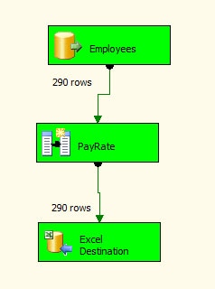
Figure 25: The data flow after if has completed running

You can also find details about the package’s execution on the Progress tab (shown in Figure 26). The tab displays each step of the execution process. If there is an error, a red exclamation mark is displayed next to the step’s description. If there is a warning, a yellow exclamation mark is displayed. We will go into resolving errors and how to find them in a future article.

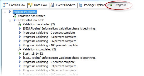
Figure 26: The Progress tab in SSIS Designer

Now all that’s needed is to check the Excel file to ensure that the data was properly added. You should expect to see results similar to those in Figure 27.

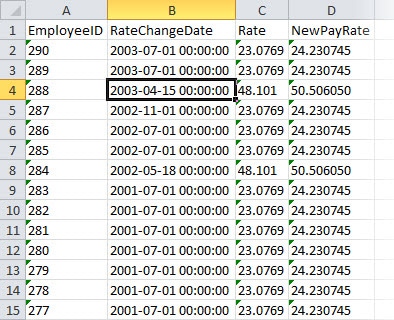
Figure 27: Reviewing the Excel file after package execution

Summary

In this article of the “SSIS Basics” series, I’ve shown you how to add the data flow to your SSIS package in order to retrieve data from a SQL Server database and load it into an Excel file. I’ve also shown you how to add a derived column that calculates the data to be inserted into the file. In addition, I’ve demonstrated how to run the package.

In future articles, I plan to show you how to deploy the package so you can run it as part of a scheduled job or call in other ways. In addition, I’ll explain how to use variables in your package and pass them between tasks. I also aim to cover more control flow tasks and data flow components, including those that address conditional flow logic and for-each looping logic. There is much much more that can be done using SSIS, and I hope over the course of this series to cover as much information as possible.