

Introduction
In my last article, An Introduction to Azure Data Explorer, I discussed the process of creating and using Azure Data Explorer. Azure Data Explorer is mainly used for storing and running interactive analytics on Big Data.
First, I need to create the ADX cluster. Then, one or more databases should be created inside the cluster. I may create one or more tables with columns under each database to populate data. Complex analytical queries are written on the table data using Kusto Query Language (KQL). KQL offers excellent data ingestion and query performance. KQL has similarities with SQL language as well. KQL allows to write data queries and control commands for the database and the database tables.
In this article, I will discuss about the basics of KQL and will write some queries to get familiar with the usage.
Kusto Queries
Kusto Query is a read-only request to process data and return the result of the processing. No data or metadata is modified. The query consists of a sequence of query statements delimited by a semicolon (;). One of the query statements should be a tabular expression statement. This tabular expression statement returns the result of the query in a row-column format.
Query Statement Types
Query statements are of two types: user query statements and application query statements.
User query statements are statements primarily used by the users. The different user query statements are:
- let statement: used to break a long query into small named parts for easy understanding.
- set statement: sets a query option to define how the query is processed and the query result is returned.
- tabular expression statement: returns data as result in a tabular format
Application query statements are statements designed to support scenarios in which mid-tier applications take user queries and send a modified version of them to Kusto. The different application query statements are:
- alias statement: defines an alias to another database in the same cluster or different cluster
- pattern statement: used by applications to inject themselves into the query name resolution process.
- query parameters statement: used by applications to protect themselves against injection attacks
- restrict statement: used by applications to restrict queries to a specific subset of data in Kusto
Example Kusto Query
In the below query, there are two statements separated by a semicolon; The first one is a set statement to enable query trace for this particular query. The second statement is a tabular expression statement, which returns the count of records from the ls1 table as a result data after the query execution.
set querytrace;
ls1
| count
Other Features of Kusto Query
A Kusto query is a read-only operation to retrieve information from the ingested data in the cluster. Every Kusto query operates in the context of the current cluster and the default database of the current cluster. It is possible to write cross-database and cross-cluster queries also. To access tables from any database other than the default database, read permission should be available. To execute cross-cluster query, the cluster that is doing the initial query interpretation must have the schema of the entities referenced in the remote clusters. The details about cross-database and cross-cluster queries are not discussed in this article.
Individual Kusto queries can be written and executed. Also, Kusto supports different types of functions which are good for reusable queries. Functions will be discussed in separate article.
Control Commands
Control commands are used to process and modify data and metadata in the ADX database. Control commands are not part of KQL syntax. A control command starts with the dot (.) operator, which differentiates it from the Kusto queries. The distinction between queries and control commands helps in preventing security attacks as the control commands cannot be embedded in the Kusto queries.
There are some control commands that are used to display data or metadata. These commands start with .show.
Implementation of Kusto Queries and Control Commands
I will create an ADX cluster and a database under the cluster. Then, I will ingest data in a table in the database from a CSV file. Then, I will write some Kusto queries and control commands on the table and its data. I will provide all the necessary details to complete the required tasks at each step.
Create the Azure Data Explorer Cluster and Database
An Introduction to Azure Data Explorer may be referred for the step-by-step process of data ingestion from a CSV file to the ADX database table. I ingest data from a CSV file in my local drive to a table named ls1 in the ADX cluster created.
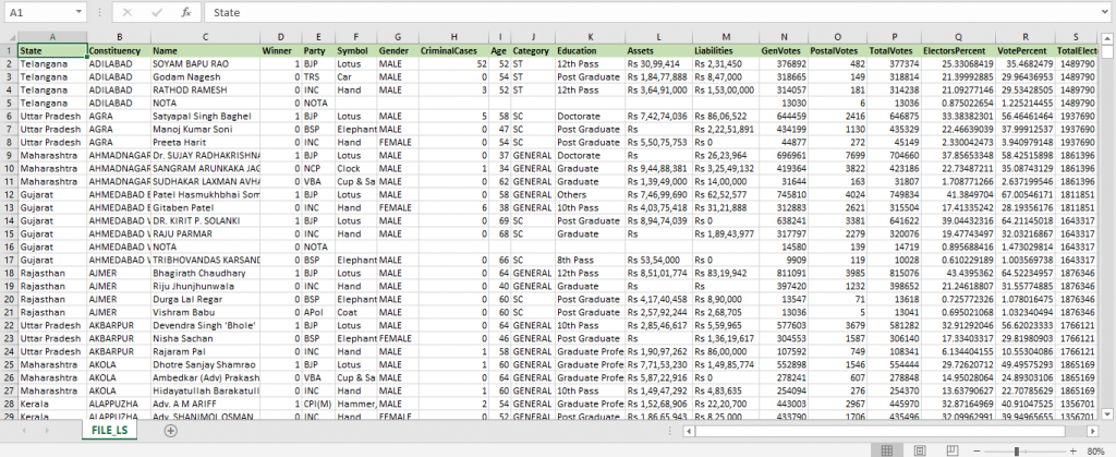
The following image shows the data file I am using here for data ingestion and writing queries. Any CSV file may be used for this exercise.
Write the basic queries on my data
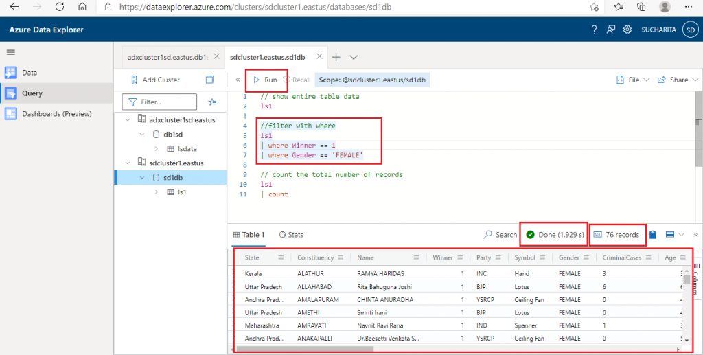
Once the data ingestion is complete, I click 'Query' in the left panel to go to the Query tab. I enter the following code and press the 'Run' button. This query should return all the records from the table ls1 having the Winner column value equal to 1.
ls1
| where Winner == 1
The result data comes in a row-column format. The time taken for the query execution and the total number of records retrieved are also displayed above the query result.
I write few other queries in the Query Window and execute them. All these queries contain only tabular expression statements.
The following query will show the entire table data from ls1.
ls1
The next query is to retrieve all the records from ls1 table applying two filter conditions. The table name and the two where conditions are separated by the pipe (|) delimiter.
ls1
| where Winner == 1
| where Gender == 'FEMALE'
In the third query, count operator is used to retrieve the total number of records from ls1 table.
ls1
| count
In the last query, where and count operator are used together to count the number of records in ls1 table where Winner value is 1.
ls1
| where Winner == 1
| count
Use a Few Common Operators
In Query 1, I use the sort, take, and project operators on ls1 table.
- sort: sort the records of the table based on the column(s) supplied in ascending or descending order. Sorting is done in descending order by default.
- take: returns only the number of records specified from the table, not the entire record set
- project: returns only the columns specified, not all the columns from the table.
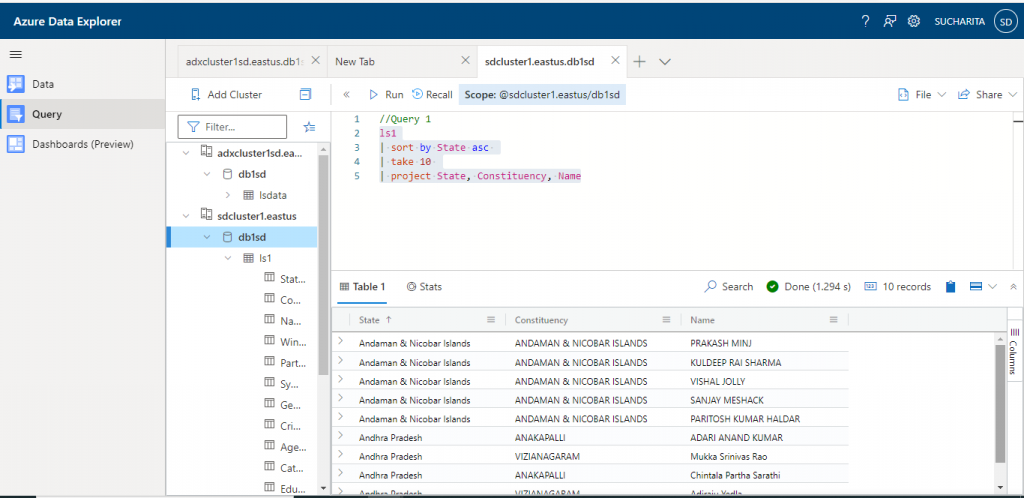
This query returns the first 10 records with the three columns State, Constituency and Name from the table ls1 sorted by State column in ascending order.
//Query 1
ls1
| sort by State asc
| take 10
| project State, Constituency, Name
The output of the query is as below:
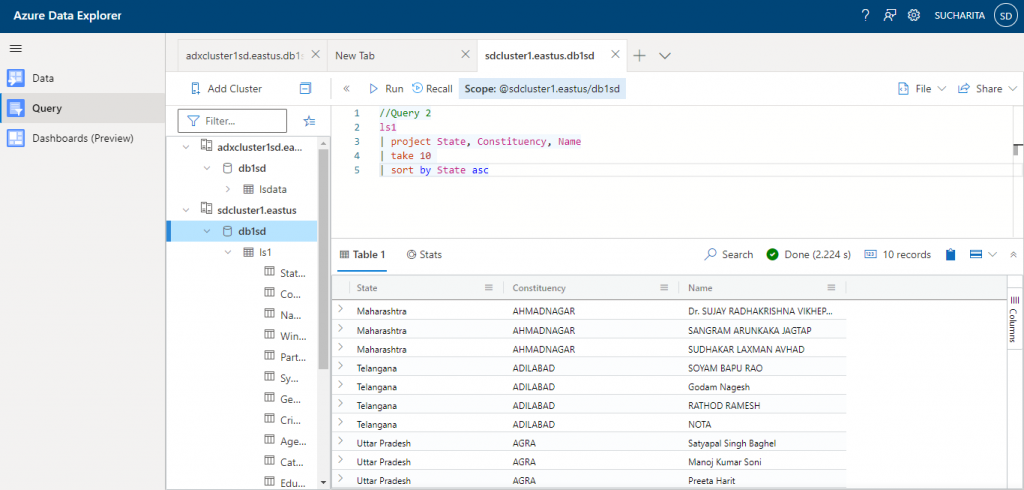
In Query 2, same set of operators are used on ls1 table, but in a different order.
//Query 2
ls1
| project State, Constituency, Name
| take 10
| sort by State asc
The change in order of operators in the query changes the output as well.
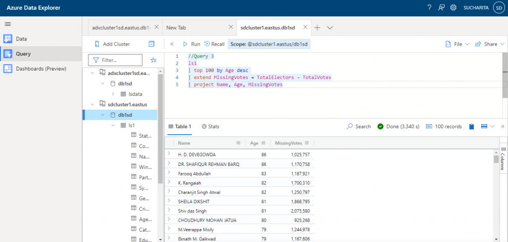
In Query 3, I use top, extend, and project operators on the ls1 table.
- top operator: this operator retrieves the number of records mentioned after sorting the dataset on the mentioned column. top 10 by Name is equivalent to sort by Name | take 10.
- extend operator: used to create a new derived column. In this query, derived column named MissingVotes is created from TotalElectors and TotalVotes columns of ls1 table.
- project operator used table columns and the derived column to retrieve data. The project operator should be used after extend operator.
//Query 3
ls1
| top 100 by Age desc
| extend MissingVotes = TotalElectors - TotalVotes
| project Name, Age, MissingVotes
Output from Query 3 is as below:
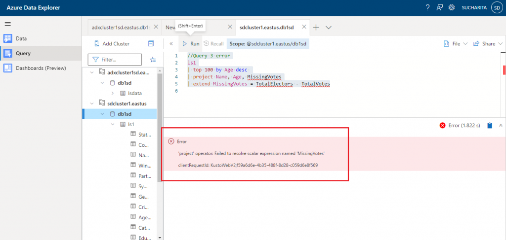
If I place the project operator before the extend operator in this query, it will give an error. Because the MissingVotes derived column is not available before the extend operator is executed.
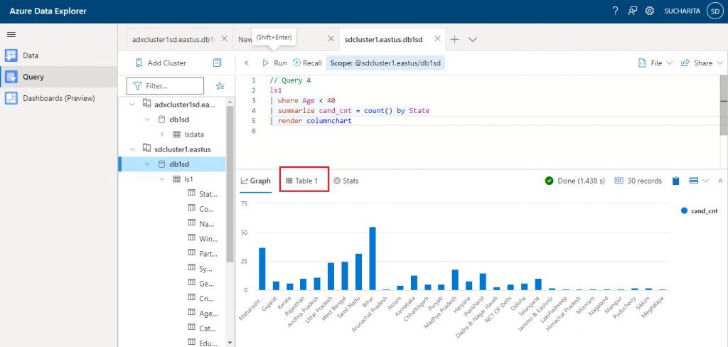
In Query 4, I use where, summarize, and render operators on ls1 table.
- where operator: this is used to filter the records from the table based on Age value less than 40.
- summarize operator: Input rows are arranged into groups based on the values of the column as mentioned with the by clause. Then, the specified aggregate function is executed on each group and produces one row for each group.
- render operator: it is used for generating Data Visualization from the query result data. Render should be the last operator in the query and used only with queries that produce a single tabular data stream result. There are different visualization options available to generate the graphical output of the query.
// Query 4
ls1
| where Age < 40
| summarize cand_cnt = count() by State
| render columnchart
The result of Query 4 is as below. The diagram shows the graphical output from the Kusto query where the render operator is used. Here, the number of candidates in each state is counted with the summarize operator and then the data is displayed with a column chart. The output data in row-column format is also available in the Table1 tab.
Control Commands
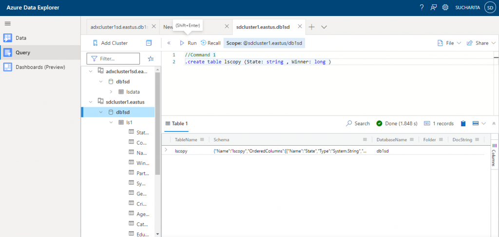
Now I use some control commands in the database. Command 1 is used to create a new table named lscopy having two columns: State and Winner.
//Command 1
.create table lscopy (State: string , Winner: long )
The output shows the structure of the new table created.
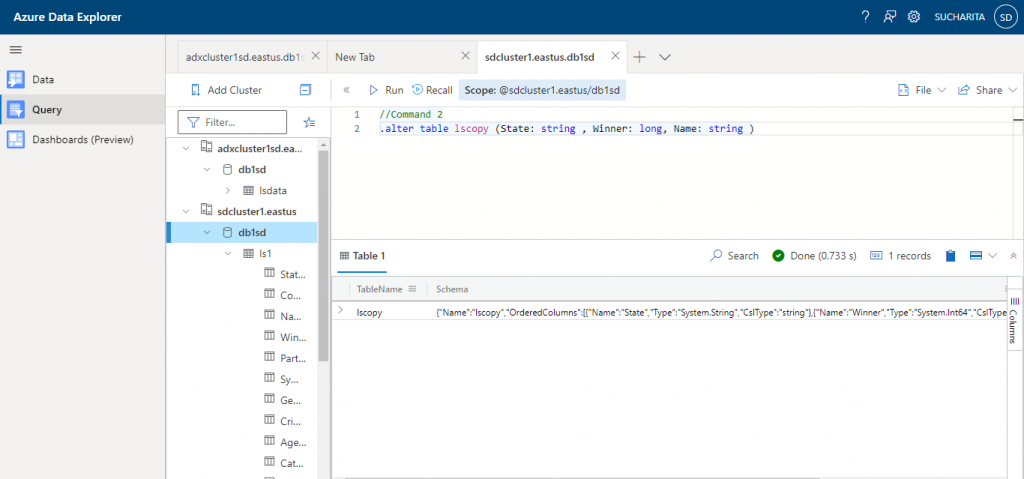
Command 2 is used to modify the existing table structure of lscopy. Here, I am adding a new column named Name in the table.
//Command 2
.alter table lscopy (State: string , Winner: long, Name: string )
The output shows the structure of the modified table.
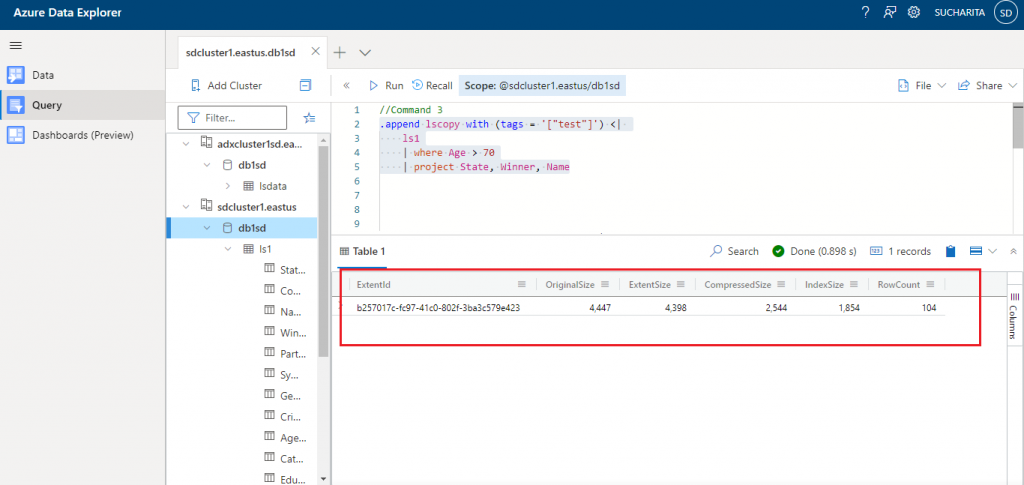
Command 3 is used to add records in the new table lscopy from another existing table ls1 based on the filter condition of Age greater than 70. Data for the columns State, Winner and Name are copied.
//Command 3
.append lscopy with (tags = '["test"]') <|
    ls1
    | where Age > 70
    | project State, Winner, Name
The output shows that 104 records are appended in lscopy table from ls1.
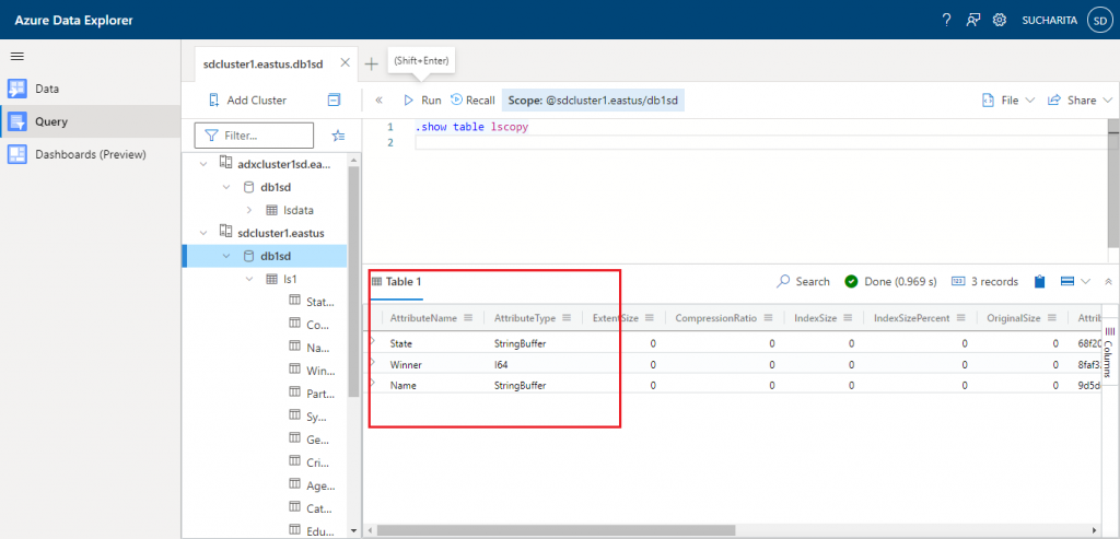
Command 4 shows the structure of the table lscopy.
//Command 4
.show table lscopy
The output is as given below:
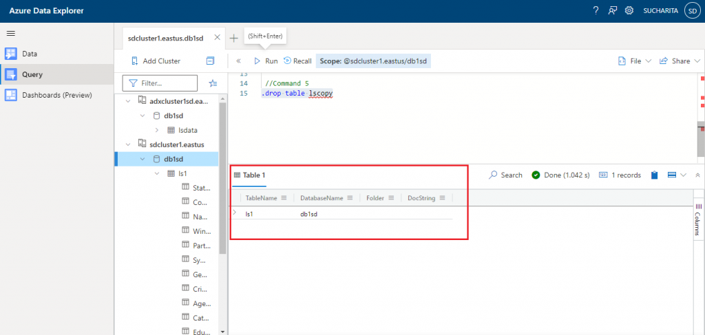
Command 5 is used to drop the table lscopy.
//Command 5
.drop table lscopy
The output shows only the tables existing in the database. ls1 is listed.
Join operator
The Join operator is used to merge the rows of two tables to form a new table by matching values of the specified columns from each table. The left table is known as outer table and denoted as $left. The right table is known as inner table and denoted as $right.
In Query 1, after on clause, only the column name State is mentioned as this same column name is available in both the tables. But, in case we need to compare the columns from the two tables having different names, it should be mentioned as: $left.State1 == $right.State2
After the join clause, kind parameter may be used to mention the type of join. Default type of join is inner join.
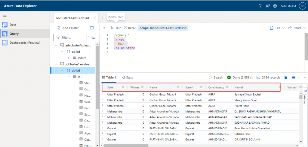
//Query 1
lscopy
| join
ls1 on State
The output is as given below for the inner join between lscopy and ls1 table on State column (present in both the tables).
The columns having the same name in the two tables are displayed with a suffix 1 for the right table. The State column is displayed as State1 for ls1 to distinguish it from the State column of lscopy table.
In Query 2, filter conditions are added after the join clause to filter the output records based on the filter conditions mentioned.
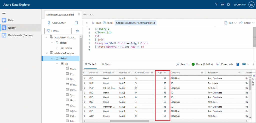
// Query 2
ls1
| join
lscopy on $left.State == $right.State
| where Winner1 == 1 and Age == 58
The output is as given below:
Records with Age = 58 and Winner1 = 1 values are only retrieved in the resultset.
In Query 3, the join kind is specified as leftouter to do the left outer join between ls1 and lscopy tables.
//Query 3
ls1
| join kind = leftouter
lscopy on $left.State == $right.State
| where Age == 58
The output is as given below. For the records that are only present in ls1 but not in lscopy table, the lscopy column values are coming as blank in the output dataset. Here, left outer join happened between ls1 and lscopy table on State column.

Conclusion
Kusto Query Language is used to query large datasets in Azure. Besides Azure Data Explorer, it is commonly used to query data from other services like Azure Application Insights, Azure Log Analytics and Azure Monitor Logs. Structured, semi-structured (JSON like nested types) and unstructured (free-text) data can be processed using KQL. This is easy to write and similarity with SQL language helps to learn quickly. I have discussed the basics of KQL in this article to start working on Azure Data Explorer. Detailed discussion about Kusto Query Language may be done in upcoming articles.