U-SQL can be used to pull data from files and tables. Previously, we’ve used U-SQL to pull data from a single postcode file, with the query below doing the heavy lifting for us

@results = EXTRACT postcode string,
total int,
males int,
females int,
numberofhouseholds int
FROM "/Postcode_Estimates_1_M_R.csv"
USING Extractors.Csv();
@m12results = SELECT postcode, total, males, females
FROM @results
WHERE postcode.Substring(0, 3).ToLower() == "m12";
OUTPUT @m12results TO "/output/M12Postcodes.csv"
ORDER BY total DESC
USING Outputters.Csv();

But U-SQL is capable of much, much more. Instead of working on one file, it can work concurrently on multiple files, providing fast access to potentially billions of rows. We’re going to write a query to access multiple files – hold on to your hat!

The Data

We’re again going to use data from the Office of National Statistics. If you haven’t already pulled the files down, head on over to the ONS Web site and grab the Postcode Estimates file. You will find eight CSV files in the zip file – we’re going to work on four of these, all beginning with Postcode_Estimates_2. These files contain four columns:

• Postcode
• OA_Code
• Total
• Percentage

The same OA code (OA means Output Area) can appear in more than one file. We want to write a query which will return the total number of records for each OA Code.

Preparing The Data

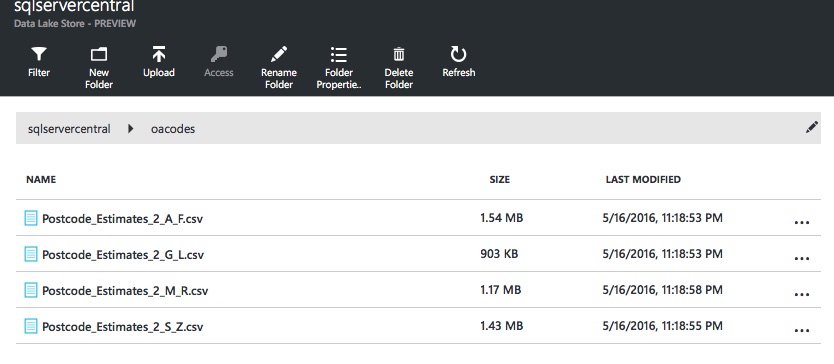
If you’ve already worked through the previous tutorial, you will be aware that U-SQL currently doesn’t handle header rows very well (UPDATE February 2017 - U-SQL now supports header rows). So before we do anything else, open up the four Postcode_Estimates_2 files and remove the headers from them. Next, we need to put these four files into a folder of their own. In an ideal world we’d be able to filter on partial file names, but U-SQL only supports wildcard querying at the moment. So open up your Azure Data Lake Storage account, create a folder called oacodes, and upload the four headerless files into the new folder.

Now we’re ready to go!

The Query

The query to process multiple files doesn’t look hugely different from our single file query:

  @results = EXTRACT postcode string,
  oacode string,
  total int,
  percentage int,
  filename string
  FROM "/oacodes/{filename:*}.csv"
  USING Extractors.Csv();
  
  @oacoderesults = SELECT oacode, COUNT(*) AS total
  FROM @results
  GROUP BY oacode;
  OUTPUT @oacoderesults TO "/output/oacode_totals.csv"
  ORDER BY total DESC
  USING Outputters.Csv();

You may have expected the EXTRACT statement to specify four columns, but it actually specifies five – what is this madness, I hear you cry! Fret not, for it’s not madness you’re seeing. What you’ve encountered is a rather cool U-SQL feature called Virtual Columns.

Virtual Columns

You can specify dynamic filenames in U-SQL using wildcards or dates. Date formats can be specified and U-SQL will process files that match the date pattern. You can return these filtered values as virtual columns. Look at the FROM line in our EXTRACT statement:

  FROM "/oacodes/{filename:*}.csv"

The path includes the curly bracketed value {filename:*}. Filename is the name of a virtual column, which, you guessed it, will store the filename in which the processed row was located. We’ve told U-SQL to pull back any files in the oacodes folder with a .csv extension.

As much as I tried, I couldn’t make U-SQL recognise a partial file name, e.g.:

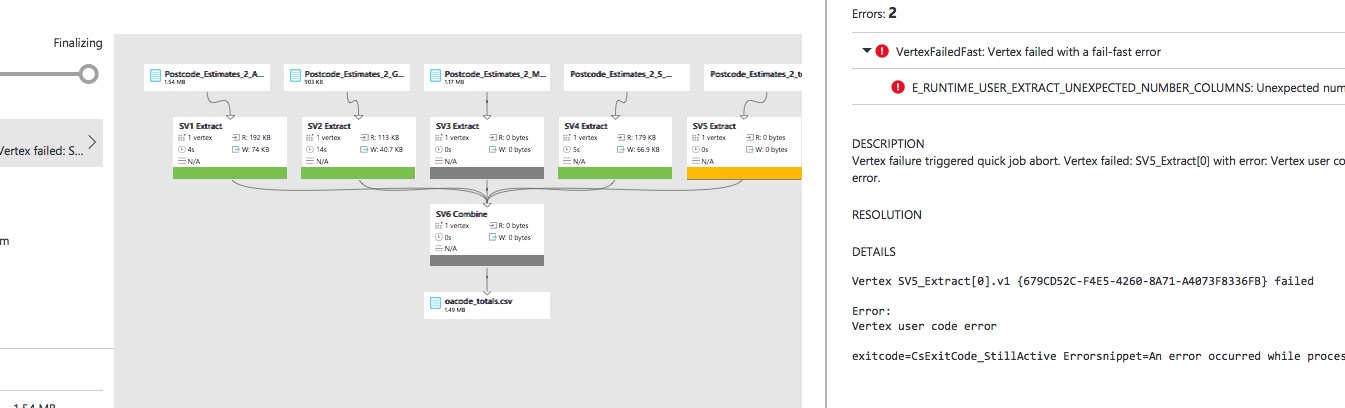
  FROM "/oacodes/postcode_estimates_2{filename:*}.csv"

Samples provided by Microsoft use similar layouts, so we'll presume this feature needs more testing at the time of writing. Anyway, at this point we’ve successfully told U-SQL to work on all files matching the pattern, so we can proceed. It’s worth pointing out that all files that match the wildcard pattern must have the same structure, otherwise our U-SQL statement will fail – here’s an example of what you’ll see should this occur (look at the unexpected number of columns error in the top right-hand corner):

Aggregation

Much of the rest of the query is stuff we’ve seen before. The only remaining point of interest is to check out the SELECT statement, which totals up the OA Code values:

  @oacoderesults = SELECT oacode, COUNT(*) AS total
  FROM @results
  GROUP BY oacode;

If you’re thinking this looks virtually identical to a T-SQL statement, you’d be right! U-SQL supports a number of typical aggregation functions, like COUNT(), AVG() and MAX(). The full list is available via MSDN. GROUP BY is also supported, and it is fully featured – so you can add HAVING clauses too. We could enhance the statement above to only return OA Codes with a count of ten or more records:

  @oacoderesults = SELECT oacode, COUNT(*) AS total
  FROM @results
  GROUP BY oacode HAVING COUNT(*) >= 10;

If we wanted to return OA Codes with a count of, say, 14, you’d notice the C# equality operator is used, not the T-SQL version:

  @oacoderesults = SELECT oacode, COUNT(*) AS total
  FROM @results
  GROUP BY oacode HAVING COUNT(*) == 14;

Executing the Query

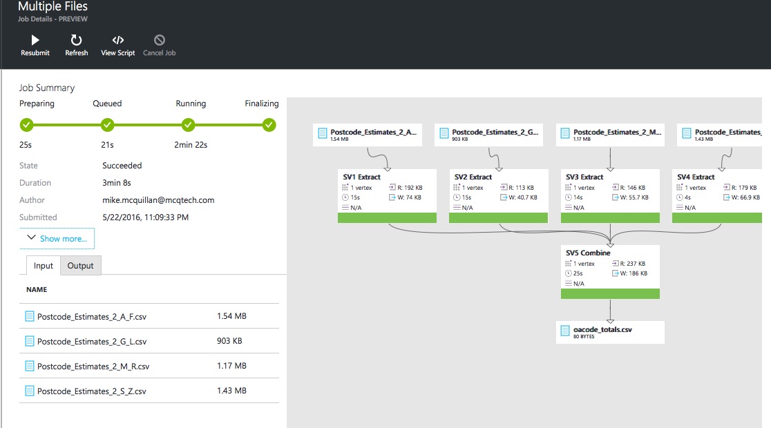
In the image below, I’ve executed the query without a HAVING clause (remember, to execute the query via the Azure Portal, open your Data Lake Analytics account and click the New Job button to enter the query). Note the execution map that is generated – it shows the four files matched and processed. The query takes a couple of minutes to run (remember, U-SQL is a batch job language designed for millions or billions of rows – if you want instant results go back to SSMS and SQL Server).

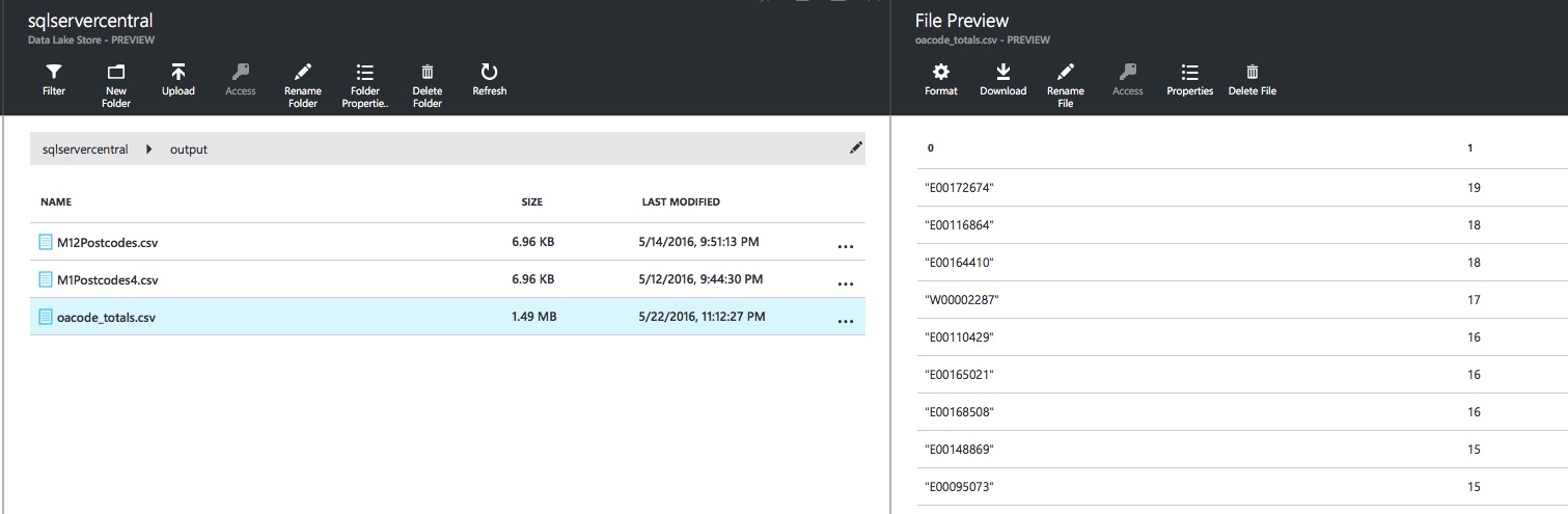
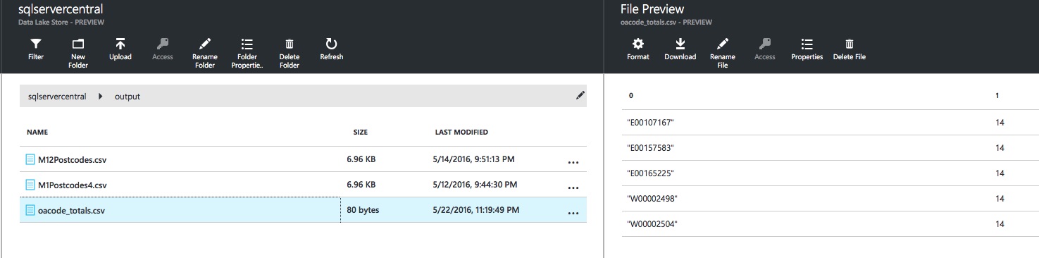
After the job completes, pop over to the output directory specified in the OUTPUT statement and open the oacode_totals.csv file. You’ll see some lovely OA Code total goodness, ordered by COUNT(*) descending as requested:

If we had executed the version with HAVING COUNT(*) == 14, we’d only see OA Codes in the file with a count of 14:

Powerful stuff!

How It Works

When processing even a single file, U-SQL splits it into something called an extent. This is not an extent as you might think of it in SQL Server, but the concept is similar. Each extent holds a number of rows. This is done to parallelise execution and speed up query processing. As with Google BigQuery, the speed of the platform comes from mass parallelism. Multiple extents are executed on individual nodes, with the results being returned and amalgamated to produce a final result set.

Summary

We’ve seen another example of how powerful U-SQL is. Thanks to its wildcard filtering capabilities, we can process multiple files as one big data set. We’ve also had an introduction to aggregation, with the COUNT and GROUP BY keywords.

Next time, we’ll look at how we can use Visual Studio, instead of the Azure Portal, to process our U-SQL queries. This gives us a much better development experience and access to some cool tools.