
Introduction
Partitioning in Analysis Services (SSAS) is an option to help with nightly processing. Processing new data in a fact table rather than the whole table will save time. An easy structural change can be made on large transaction tables. The partitioning option enables the data to be separated in partitions and a date column is one of the best partitioning options. Every table in a tabular model is a single partition by default. The advantages will be seen when a fraction of the data is processed compared to the whole fact table.
Fact tables
In a dimensional model, the tables with the most data are usually the fact tables. Even though dimension tables can get large, the main focus on partitioning is on fact tables. The World Wide Importers DW database contains at least 2 tables used in previous articles that are facts: Sales and Transaction (Figure 1).
NOTE: If following from the first article, the Sales fact table might be named Sale. This article uses Sales as the table name.
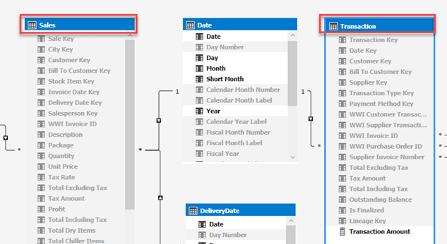
Figure 1 Sales and Transaction tables
The Sales table can be partitioned by Invoice Date Key and the Transaction table by Date Key. Since these are a Date data type, we can select groups of data in 2 or more partitions. The first in this example will be any data less than a certain date like 01/01/2014. The second partition can be a range of dates like 01/01/2014 thru 12/31/2015. The last partition will be everything from 01/01/2016 to the present called the current partition.
| Partition | Range |
| 1 | < 2014 |
| 2 | Between 2014 and 2015 |
| 3 (Current) | >2015 |
Table 1 Partitions
Partitions
To partition a table in SQL Server Data Tools (SSDT), the project and model needs to be open like in Figure 2.
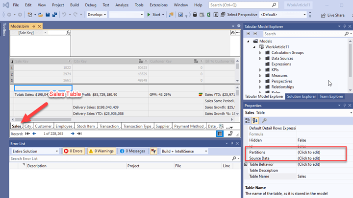
Figure 2 Project and Model opened in SSDT
NOTE: If following from the first article, your project might have been created in SQL Server Data Tools (SSDT) 2017 in a previous edition of the Analysis Services extension. This article assumes you are using SSDT 2019 with the latest Analysis Services extension. To get the same Design screen as below, you might have to click the SQL button first to see the Design button. Otherwise, create a new project in SSDT 2019 with the latest Analysis Service extension. Make sure the Model is in the latest compatibility mode before connecting to the database and importing tables.
In the properties of the Sales table, the Partitions property can be selected with the ellipse on right. This will bring up Figure 3 (Partition Manager).
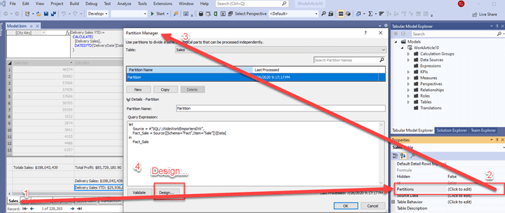
Figure 3 Partition Manager
From the Partition Manager, select the Design… button (Figure 3) on the bottom left to edit the Partition. Every table is a single partition when created. Figure 4 shows the Power Query Editor after clicking the Design… button. The screen has been widened in order to see the Invoice Date Key column. The bottom right also has an Applied Steps list that shows the changes made in Power Query (generating M Code).
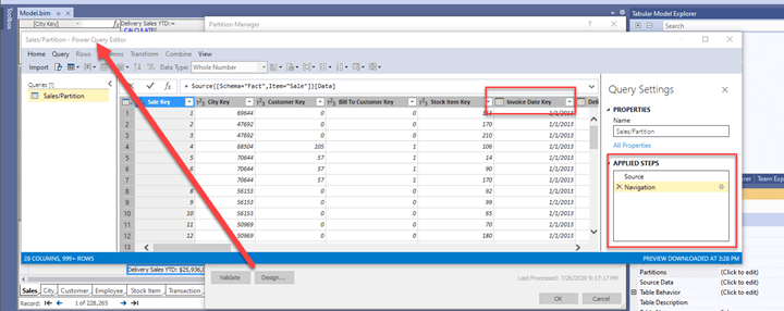
Figure 4 Power Query Editor
In order to limit the first partition data, select the drop-down arrow to the right of the Invoice Date Key column (Figure 5). This will enable a menu (Figure 5) to use the Date Filters option.
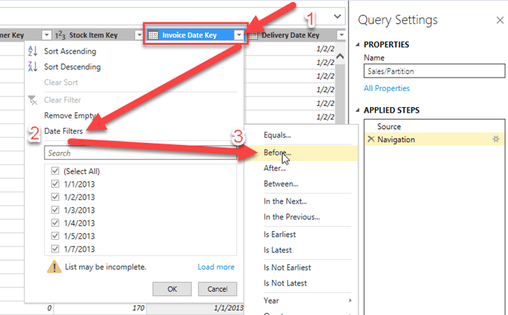
Figure 5 Date Filter
After clicking the Before… menu choice, the Filter Rows screen will appear (Figure 6). Enter 01/01/2014 in the text box or select the date with the Date selector to the right. After Ok is clicked, there will be a new row in the Applied Steps list.
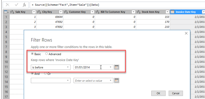
Figure 6 Filter Rows
Right click on the Filtered Rows item in the Applied Steps (Figure 7) and rename to “InvoiceDate before 2014”.
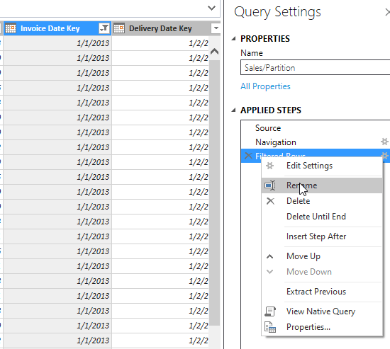
Figure 7 Rename Applied Steps
In order for the changes to be applied, click the Import button in the top left of the Power Query Editor like in Figure 8.
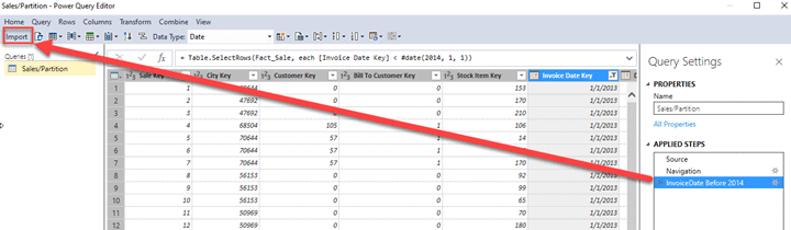
Figure 8 Power Query Editor – Import
The Import will include a new line of M code in the Partition Manager (Figure 9). Also, rename the partition ‘Sales Before 2014’. We will use this partition to copy for other partitions.
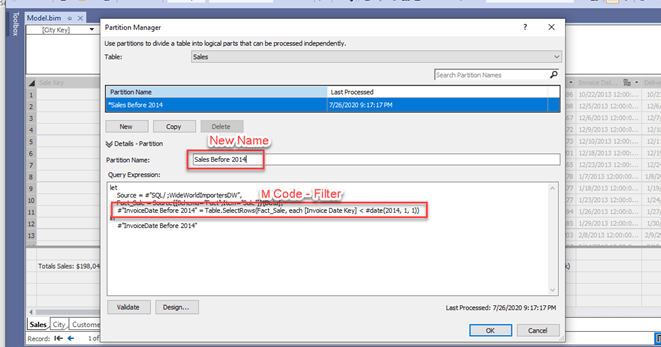
Figure 9 Filtered Partition
It is always a good idea to save the solution after making some changes. So, after clicking OK in Partition Manager Screen (Figure 9), save the solution from the file menu or the save button on the tool bar.
To create the next partition, go back into the Partition Manager from the Partition property ellipse. Click the Copy button (Figure 10).
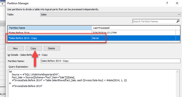
Figure 10 Partition Manager – Copy
This will add a new row in the table and the copy will have the name “Sales Before 2014 – Copy”. Rename to “Sales between 2014-2015”. With the row highlight, click the Design… button in the lower left. Figure 10 shows a part of the Power Query Editor. Instead of clicking the drop-down to the right of the Invoice Date Key column, click the Settings icon to the right of the “InvoiceDate Before 2014” item in the Applied Steps list (Figure 11).
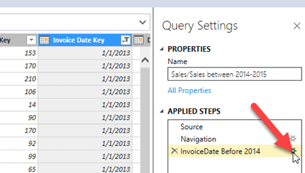
Figure 11 Applied Steps
Figure 12 shows the changes – “is after or equal to” (1/1/2014) and “is before or equal” (12/31/2015). There are lots of options for filters, so most if not all scenarios can be satisfied.
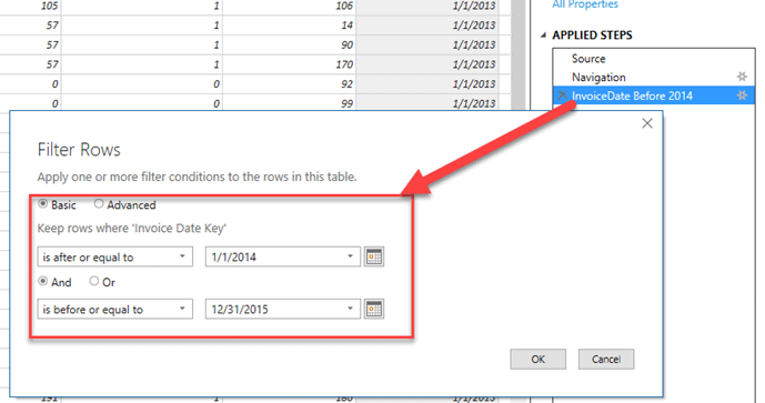
Figure 12 Filter Rows – Sales Between 2014-2015
After clicking ok, right click the filer item (“InvoiceDate before 2014”) in the Applied Steps to rename “Sales between 2014-2015”. Click the Import button in the upper right to get back to the Partition Manager.
Click Copy again to create the last partition – Sales after 2015. This will be the current partition where data has the possibility of changing in the source database. It is also the partition that will be processed nightly instead of the whole table or all partitions.
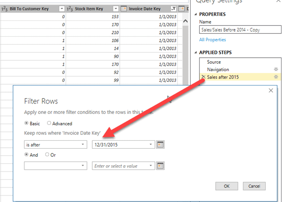
Figure 13 Filter Rows – Sales after 2015
Follow the same steps as the previous work for “Sales between 2014-2015” except rename the Applied Steps item to “Sales after 2015” and use a single filter for “is after” (12/31/2015) as shown in Figure 13. Rename the copy to “Sales after 2015” and be sure to save all the work.
Processing
The next step is to process the partitions. Figure 14 shows the Partition submenu in SQL Server Data Tools 2019 under the Extensions menu. The selections include an option for Process Partitions…, Process Table or Process All. This example is for the partitions, so select the first option “Process Partitions…”. The Process Table would be for the whole table selected. Process All would process all tables in the model.
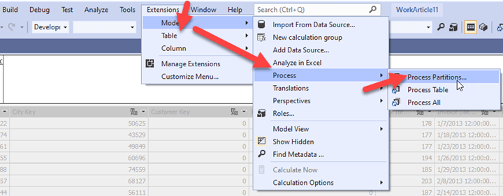
Figure 14 Partition Menu and Sub-menus
Once Process Partition… is selected, the list of available partitions will be display (Figure 15). Select the needed partitions to process and Mode: Process Full, then click Ok. The Process Modes are Default, Full or Clear/Recalc. More details of all modes will be in a different article.
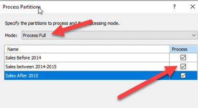
Figure 15 Process Partition
The number of rows will be by partition. The sum should be all rows in the table.
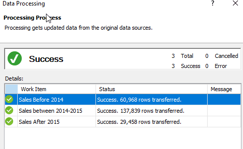
Figure 16 Processing Partitions Sales
Now, in the nightly processing, only the current partition (Sales after 2015) has to be processed and the 2 previous partitions do not. This should reduce the processing time on the model in production.
Summary
Partitions are a handy structural change that will help IT departments with processing times for a Tabular model. Full processing likely is used at the beginning of a model deployment. Over time as more and more data gets imported and new tables are added to a model, the architects will see an increase in processing times. Microsoft has done a great job with adding partitions to this model type just like with Multidimensional Cubes. The execution will take some changes to the simple Full mode job, but the payoff will be reduced processing time and maintaining Service Level Agreements (SLAs) with the business. The business appreciates readiness of available data for reporting and analysis.