Introduction

One of the more important features in Analysis Services 2000 was the ability to utilize query history to design aggregations to enable better performance for the most common queries in the organization. Analysis Services was able to determine, using specific filters the user has applied, which queries it needs to take into account when designing aggregations. Aggregations are pre-calculated summaries of data which the OLAP engine calculates during the processing of a cube. Having these summaries pre-calculated comes handy when a user is querying a cube. If the query is corresponding with a pre-calculated summary of data (an aggregation), the OLAP engine can deliver the results quicker then having to calculate the data on the fly. When a developer creates aggregations for the first time, then obviously there is no query history available for that cube. The OLAP engine treats each possible query the same, meaning each query has the same "chance" to be executed by a user. This is, of course, not the case in the real world, where users are predominantly querying the cube the same set of queries each and every day. This is where using the usage-based optimization wizard makes real sense.

The Query Log Table

In a previous article I have explained how to enable query logging in SSAS 2005. By doing so you instruct the OLAP engine to log the queries executed on its databases to a log table. This table is used when designing aggregations based on query history. Let's have a look at the table's content:

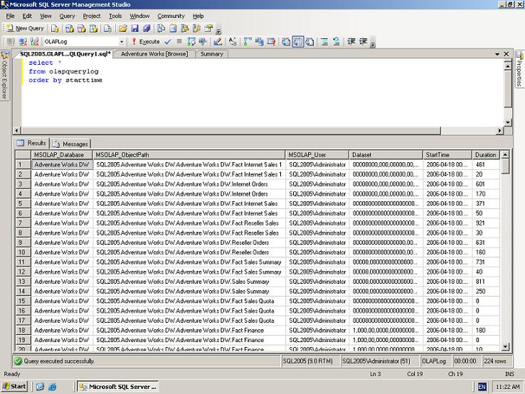
The first column: [MSOLAP_Database] indicates the database the query is being executed on. The second column: [MSOLAP_ObjectPath] describes the path to the specific measure group being queried, in the following structure: [Server ID].[Database ID].[Cube ID].[Measure Group ID]. The third column: [MSOLAP_User] is simply the user running the query. The fourth column: [Dataset] represents the dimensions and measures taking part in the query. The representation of the objects participating are not self describing. The fifth column: [StartTime] is the execution start time and the sixth, last column: [Duration] represents the duration of the query. The OLAP administrator does not need to view this table's content, as it is used internally by the OLAP engine to store query execution history only, which later will be used by the usage-based optimization wizard. I just thought it would be interesting to understand how the OLAP engine is storing this data.

Running the Usage-Based Optimization Wizard

Now that we understand how to enable query logging and we had a sneak peek at the log table's content we are ready to start using the Usage-Based Optimization wizard. Firstly, we obviously need to wait for some data to accumulate. We want to let the users query the cube for a certain period of time, which we think is representative of the average workload for that cube. This could range from a day up to a month, depending on the organization. Once we have the data collected we can start the wizard. You can do so in two ways, either right-click on a specific partition within a cube using the SQL Server Management Studio (SSMS). Alternatively, you can use the "Partitions" tab on your Business Intelligence Development Studio (BIDS) when you are editing an online database. On that tab simply click the "Usage Based Optimization" icon on the toolbar. Make sure you have clicked on one of the partitions first, otherwise this option will not be available to you.

Option 1 - Using SSMS

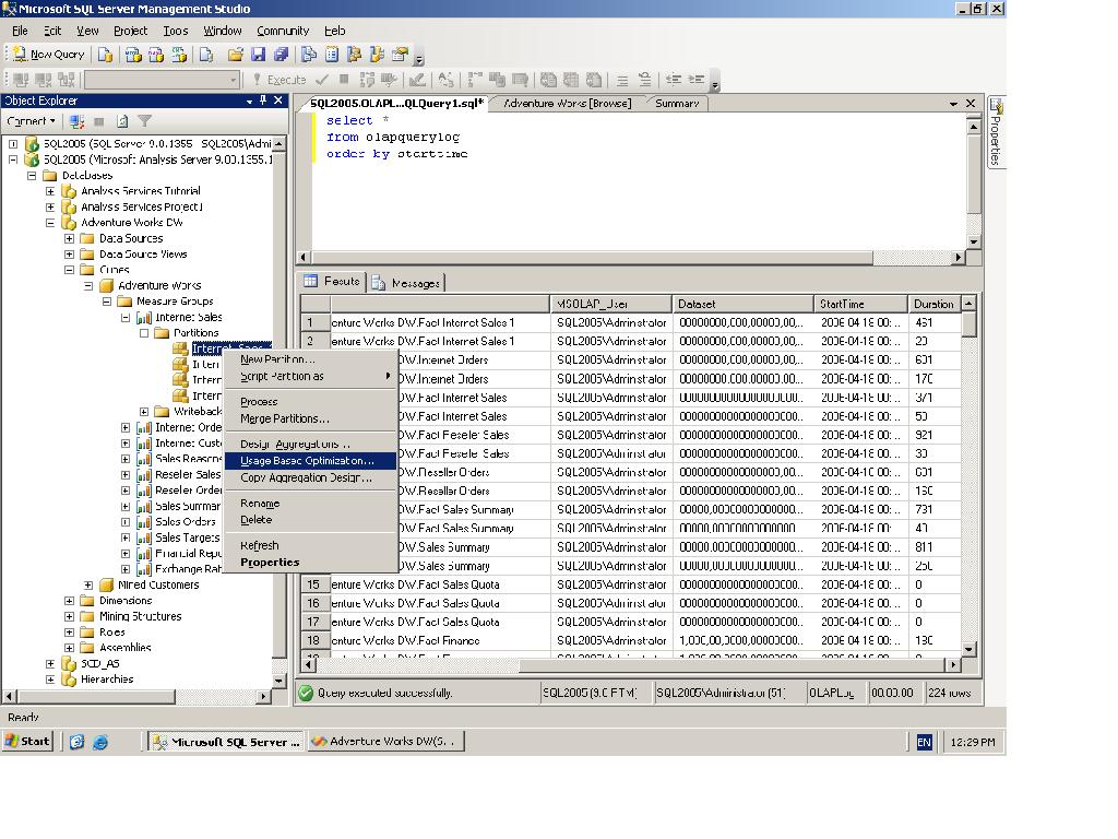
Option 2 - Using BIDS

Once we kick-started the wizard we will receive the "Welcome" screen:

Clicking "Next" will bring us to the next screen:

Here we can view how many queries are stored in our log table, how many distinct queries are there, and how many users have queried the relevant partitions. Another important figure we can gather from this screen is the average query duration. Now we need to decide if, and how we want to filter the data stored in the log table. We have several options to do this, and we can combine one or more options in one filter. We have the option to filter the queries according to a date and time. We can also filter the queries submitted by a specific user or several users. Lastly, we can choose to pick specific queries which represent a certain percentage of the entire set of queries stored in the log table. By doing so we can design aggregations specific to the most used queried.

After choosing the filter criteria, clicking "Next" will lead us to the next screen of the wizard, which simply displays the queries which comply with the filter criteria we previously set up.

Here, you can uncheck any query you do not want participating in the aggregations calculation.

Click "Next" and you will be presented with the next screen, the "Storage and Caching options" screen. From this point onwards, the steps involved in designing the aggregations are similar to designing regular aggregations. We will stick with the standard MOLAP storage options this time, as discussing the storage options in SSAS 2005 is really a major topic by itself. Suffice to say that using the MOLAP option will provide best performance for cube readers (in the most simplistic approach).

Our next step will be to count the number of records in the relevant partition and the related dimension members. This enables the OLAP engine to better estimate the size of the aggregations to be calculated, a parameter which we will need to consider in our next step. This is maybe a good point to explain how aggregations are stored. As mentioned earlier, aggregations are pre-calculated summaries of data within a cube, for example, the summary of a specific measure (i.e. "order count") within a certain dimension slice (i.e. the "Time" dimension in the "Year" level and the "Customer" dimension in the "Country" level). The aggregations are stored as files in the relevant partition folder. Aggregation size is a direct derivative of the number of aggregations designed and the size of the underlying tables (fact tables and dimension tables).

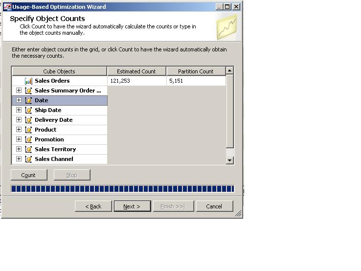
You can either click on "Count" and let the OLAP engine count the number of records in the tables, or you can simply write the number of records yourself in the designated cells. Unless it is a major hassle, it is better to let the server count the records, as you will probably get the most accurate, up-to-date picture of the underlying tables.

We have now reached the core of the aggregation design process, which is to let the server actually design the relevant aggregations.

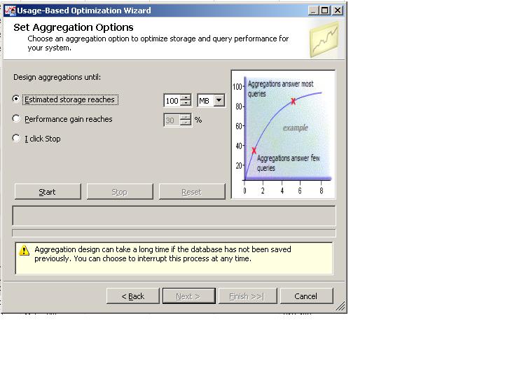
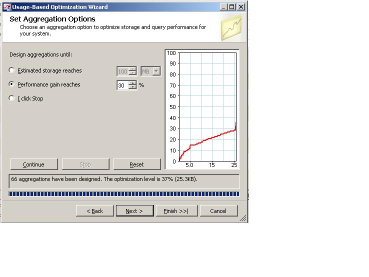
We have several options in the way of instructing the server how to design the aggregations. We can either instruct the server to limit the number of aggregations to a maximum of a certain file/s size. This way we can control the size of the aggregation files, which can become quite large in big cubes. Alternatively, we can instruct the server to calculate aggregations up to a certain percentage, which represents a performance gain. In simple words this means that, suppose we choose a value of 30%, the server will calculate aggregations which will contribute to a 30% performance gain, in contrast to those aggregations not being present in the cube. You have to take into account that the higher the percentage value is, the more aggregations will be designed, thus making the aggregation files larger and larger. The third option to choose from is until "I Click Stop". This literally means that the server will calculate more and more aggregations until the user will hit the "Stop" button. The user needs to make an educated "guess" here as to how many aggregations to design. If one chooses to design aggregations which will improve performance by 100% (as many aggregations as possible), this may mean an extremely lengthy process for large cubes, sometimes days to design and even more time to process the cube. More often then not, it is not required to design aggregations which will provide a 100% performance gain. This is because the OLAP engine is smart enough to rely on existing aggregations to derive values for related queries. For example, suppose we have designed aggregations in a "City" level in the "Customer" dimension. If a user will query the cube and ask for data at a "State" level, the OLAP engine will be able to quickly calculate these figures using the aggregations based on the "City" level. As a developer, you need not worry with regards to these types of optimizations, the OLAP engine does it for you, using internal algorithms.

As a general rule of thumb, when you initially design aggregations you want to choose the 30% figure and later use the usage-based optimization wizard to refine this design. Clicking the "Start" button will kick-start the design process and you will be able to examine the progress of the process on-screen.

We are now at the final stage of the process, after clicking "Next" once the aggregation design process is complete. We are prompted to save the new aggregations and we have the option to process the cube if we want to.

Conclusion

By designing aggregations based on query history we enable the user to quickly and efficiently retrieve data from a cube. This SSAS feature is important and is considered one of the main advantage points for SSAS 2005, compared with other OLAP engines out there in the market. In a coming article I will discuss aggregation design more thoroughly.