Introduction

One of the questions a retailing business at some point will certainly ask is: which of my products are often purchased together? We, being the SQL people, probably can wrench the answer by brute force alone, counting all permutations of product pairs and ranking them. Unfortunately, it escalates quickly to the very tedious script writing and resource consuming computations with the increasing amount of orders and products. What if could use some math magic hidden in R packages? Given that R is now a part of the SQL Server Machine Learning services, naturally, we can't wait to get our hands on the power of R inside SQL Server.

To follow this article you will need the Microsoft AdventureWorks sample database. Simply download one of the Data Warehouse backups from here. Don’t worry – they are small. Also, you will need to have R services installed on your SQL Server. As there are many excellent tutorials on how to do that, I will not provide the installation details here, and will assume that you have it installed (we have a Stairway to help). Though, please make sure that you have everything set and running before proceeding any further.

The Approach

What do we exactly want R to do for us? Well, we would like it, somehow, to group orders with the same products together. But how?

Imagine for a moment that we have a set of objects, each with a bunch of attributes: a1…aN. Now, we could use the attributes as “coordinates” in the Euclidean sense and try to apply some clustering algorithm to separate objects into groups. Obviously, objects in the same group/cluster are closer to each other than to objects in other clusters. Could we do the same to our products instead of abstract objects? In that case we would instantly have had the answer to our question. Well, we can surely calculate the distance between the objects in our abstract “attribute” space, but what on Earth is the distance between products?!

Apparently, we need to construct a space. Imagine an array of binary values. Each element in the array represents a sales order from our database. We set the value to 1 (“on”) if the product P was purchased, and to 0 (“off”), if it’s not. Now, let’s repeat it for every product we are interested in. We should end up with a matrix where each row represents a product purchasing “bitmap”, a column per order. Can we calculate the distance between the rows now? To answer that, let’s have a look at standard R function for calculating distances - dist().

Dist() expects a matrix as an argument, and, by default, calculates the Euclidean distances between the rows and returns the matrix of calculated values. Using Euclidean geometry is not the only way to calculate the distance though. At a closer look at the available methods, we will find “binary” among them. That should be helpful, since we have the matrix of binary values.  The distance is defined as “the proportion of bits in which only one is on amongst those in which at least one is on”. That is “1” and “1” will result in zero distance, “0” and “1” in the maximal one (1), and the combination “0” and “0” will be ignored in the calculations.

To understand what it means for us, we need to take a deeper dive into this.  Below I will show some results from R-Studio. I used R-Studio here as it’s much quicker and convenient to run such code snippets in, but you don’t have to. For us, at the moment, only the results themselves are important. If you want to follow my steps, please use the following R script:

# our matrix
p0 <- c(0,0,0,0,0)
p1 <- c(0,0,0,0,0)
p2 <- c(1,0,1,0,0)
p3 <- c(1,1,1,0,0)
p4 <- c(1,1,1,1,0)
# build the matrix from the rows
tm <- rbind(p0,p1,p2,p3,p4)
# binary distance
d1 <- dist(tm, method = "binary")
# binary similarity 
s1 <- 1-d1
s1

Consider the following matrix:

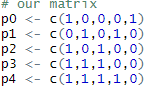
You can think that p0…p4 are the products and the columns are the orders.

Let’s calculate binary distances and convert them to binary similarities (as simple as S = 1-D, where “D” is the distance and “S” is similarity) and have a look at the values:

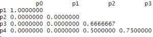
At once, we see that most similar (identical, essentially) are p0 and p1. Which, though, being true from a formal point of view, is unacceptable to us. We do not want to find that products never purchased were most often purchased together. So, in our analysis we should exclude orders that do not have the products we are interested in.

For p2, p3 and p4 everything seems is as expected. The most similar are p3 and p4. Indeed, 3 out of 5 bits are equal. Less so are the (p3, p2) and (p4, p2) pairs. But what are the values – 0.75, 0.50, and 0.6666667? By looking at the original matrix, we can easily deduce that the values are percentages of equally set columns, or orders in our interpretation, given that we excluded the elements where both values were 0. So, translating it to our language, the values will be the fractions of orders that have both products from a product pair among the orders that have at least one product from the pair. In other words, this fraction can be considered the probability of finding those two products in an order together.

The Solution

Now, that the theoretical part is over, we can start with a practical solution. One can immediately spot the potential problem – SQL Server does not support more than 1024 columns, in case you would like to use intermediate table or view. That doesn't include the fact that such an approach, converting rows to columns, would be hugely impractical. This is not a big deal, as we still can return a regular dataset where rows are orders and columns are selected products and use the awesome R matrix processing functionality to transpose the matrix, switching rows and columns.

Another potential problem, also easy to spot, would be the size of the dataset, as your Data Warehouse might contain tens or hundreds of millions of orders. Though, you still can try and test the limits of your computers using all your orders, it might be a bit wiser to choose a slightly different path. Keep in mind that all your current orders are still just a fraction of all possible ones. Imagine, that someday, everyone on Earth who has not placed an order on your website yet, starts placing orders. In theory, the results of your analysis in the future might be drastically different from what you have now. That said, you can consider all your orders as just a sample of the whole population (in statistical sense). So, why don’t you pick a smaller sample? Sure, the larger the sample, the smaller the margin of error, but this is a game of diminishing returns. In fact, to reach 95% confidence with a 1% margin of error, about 10,000 randomly selected orders is enough.

To keep things nice and tidy, we will write a stored procedure that generates the desired dataset. First, we need to find the products that comprise a pre-selected percentage of all sales (by number). You can use all products, of course, but normally, there are lots of them, which makes the results somewhat obscure. Next, we can start building the dataset. The dataset column names should be the names of the products and the values are bits indicating whether the product was purchased in the order. Writing such select statements by hand is next to impossible, as you cannot know in advance what products you are dealing with. And we will not. We will let the stored procedure do it for us. In other words, we will prepare parts of the statement such as “select”, “into”, “from” and “join” by using a well-known technique of collecting the results of a query into a string.

Note, that we need an “into” clause, because as SQL Server R InputData parameter supports only select statements, we have to download the resultset into a global temporary table. We also will be sampling the fact table by using a TABLESAMPLE PERCENT clause. You can choose any other way of sampling, but this one is designed to be fast. Further details on the stored procedure can be found in the following code snippet:

create procedure get_data_feed
as
set nocount on
declare @sample_size_percent int = 100
declare @percent_of_sales money = 50
declare @tcnt money
declare @t table(productKey int, product varchar(100), cnt int)
if( object_id('tempdb..##data_feed') is not null ) drop table ##data_feed
insert @t(productKey, product, cnt)
select f.ProductKey, p.EnglishProductName, cnt = sum(OrderQuantity) 
  from FactInternetSales f
       join DimProduct p on p.ProductKey = f.ProductKey
group by f.ProductKey, p.EnglishProductName
select @tcnt = sum(cnt) from @t 
-- select most important products
select t.productKey, t.product 
  into #products
  from (select productKey, product, cnt, cum = sum(cnt/@tcnt) over(order by cnt desc) from @t) t
 where t.cum <= @percent_of_sales/100.00
order by t.cum
-- select columns part
declare @columns varchar(max) = ''
select @columns = @columns +case when @columns != '' then ',[' else '[' end +p.product +'] = max(case when p' +cast(row_number() over(order by p.productKey) as varchar) +'.productKey is not null then 1 else 0 end)' +char(13)+char(10)
  from #products p
order by p.productKey
-- join part
declare @join varchar(max) = ''
select @join = @join +'left join #products p' +rnum +' on p' +rnum +'.productKey = f.ProductKey and p' +rnum +'.productKey = ' +cast(t.productKey as varchar) +char(13)+char(10)
  from (select productKey, product, rnum = cast(row_number() over(order by productKey) as varchar) from #products) t
order by t.productKey
-- from part
declare @from varchar(max) = '  from (select f.SalesOrderNumber, f.ProductKey from FactInternetSales f tablesample(<percent> percent)) f
       join #products x on x.productKey = f.productKey' +char(13)+char(10)
set @from = replace(@from, '<percent>', cast(@sample_size_percent as varchar(50)))
-- the other parts
declare @select varchar(max) = 'select '
declare @into varchar(max) = ' into ##data_feed '
declare @group varchar(max) = 'group by f.SalesOrderNumber'
declare @query varchar(max)
set @query = @select +@columns +@into +@from +@join +@group
exec( @query )

To wrap around the R external script execution, we also will write another stored procedure. Let’s think what we want to accomplish in the R script. First, we want to load our dataset, generated by the previous stored procedure, as a matrix and transpose it (remember, we need to switch rows and columns). Note the InputDataSet is a standard input for a SQL Server R external script:

ds <- as.matrix(InputDataSet)
tm <- t(ds)

Next, for that product/order matrix, we want to calculate the distances, again, as a matrix, as we discussed earlier:

dm <- dist(tm, method="binary")

Now, we would like to cluster the products. For this, we will be using R function hclust(), that returns an hierarchical cluster based on a matrix of distances:

hc <- hclust(dm)

Having a cluster is nice, but we need a way to visualize it. For that, we will convert the cluster to a dendrogram and plot it:

hcd <- as.dendrogram(hc, hang=0.2)
plot(hcd, main=NULL, sub="", xlab=" Distance between products", horiz=TRUE, cex.lab=0.9, col.lab="Blue")

You don’t have to use the dendrogram, the plot will draw the hierarchical cluster regardless. But the dendrogram provides a bit more control over the shape of the image (horizontal layout instead of standard vertical one, for instance). In plot() main=NULL supresses the title, and cex and col control the size and the color of the axis labels. You can have more effects for the plotting and the dendrogram with the R packages ggplot2 and dendextend respectively, but I will leave them out of the scope of this article.

Graphic output is a bit tricky when you use R with SQL Server. You want to output to a graphic file, so later on, you can read from it and return the data back to the client. For that, beforehand, you need to define the output file:

image_file = tempfile(pattern = "ROutput", tmpdir = tempdir(), fileext = ".jpg");
jpeg(filename = image_file, width = 800, height = 600);

And you need to close your device after:

dev.off();

Are we done? Not quite yet. If you don’t have an access to your SQL Server local drives, you still need to return the data (image) back to the client somehow. As I mentioned earlier, we can read the binary data right from the file we just generated. We also need to convert the data to data frame before pushing it to the client. The standard output is OutputDataSet:

OutputDataSet <- data.frame(data=readBin(file(image_file, "rb"), what=raw(), n=1e6));

Let’s put it all together to the stored procedure. Note, that we return the results as one varbinary(max) column:

create procedure [dbo].[Plot]
as
set nocount on
-- load dataset into ##data_feed
exec get_data_feed
execute sp_execute_external_script @language = N'R',  
                                   @script = N'  
    image_file = tempfile(pattern = "ROutput", tmpdir = tempdir(), fileext = ".jpg");  
    jpeg(filename = image_file, width = 800, height = 600);  
    ds <- as.matrix(InputDataSet)
    tm <- t(ds)
    dm <- dist(tm, method="binary")
    hc <- hclust(dm)
    hcd <- as.dendrogram(hc, hang=0.2)
    plot(hcd, main=NULL, xlab="Distance between products", horiz=TRUE, cex.lab=0.9, col.lab="Blue")
 
    dev.off();  
    OutputDataSet <- data.frame(data=readBin(file(image_file, "rb"), what=raw(), n=1e6)); 
   ',  
   @input_data_1 = N'select * from ##data_feed'
   WITH RESULT SETS (( c1 varbinary(max) ));

Now, the only missing part is a PowerShell script that would call the stored procedure and show us the image. The script is small and rather straightforward. Be aware that the “Start-Process” will try to start your default application for viewing jpg files:

$Source = "<Your Server>"
$Database = "AdventureWorks"
$File = "<Your folder>\result.jpg"
$conn = New-Object System.Data.SqlClient.SqlConnection
$conn.ConnectionString = “Data Source=$Source;Initial Catalog=$Database;Integrated Security=SSPI;”
$cmd = New-Object System.Data.SqlClient.SqlCommand
$cmd.Connection = $conn
$cmd.CommandText = "exec Plot"
try
{
    $cmd.Connection.Open()
    $reader = $cmd.ExecuteReader(16)
    $reader.Read()
    $bytes = $reader.GetSqlBytes(0)
    [io.file]::WriteAllBytes($File, $bytes.Buffer)
    Start-Process $File
}
finally
{
    $cmd.Connection.Close()
}

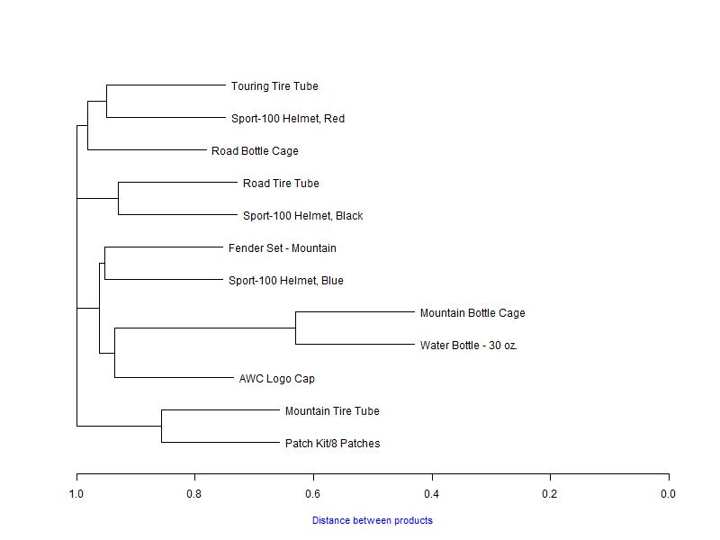
If everything worked as expected, after you ran the PowerShell script, you should have the following image:

Discussion

We can see quite a few product pairs here. Also, we can see the “Mountain Bottle Cage” and “Water Bottle - 30 oz.” pair is somewhat outstanding. So, how should we interpret what we are seeing? The urge, understandably, is to consider all the pairs we see here as true ones. But, please, don’t get carried away by the picture. Every tool has its limits.

We can, rather reliably, identify the aforementioned “Cage” and “Bottle” products as often sold together. If you remember our discussion above, about the interpretation of distance and similarity, you can see that they are sold together in approximately 37% of orders. You just need to find on the plot the distance where the fork starts, and subtract the value from 1.0. The closer the pair to the left, though, the less confident we are that it’s a true pair. We still can probably consider “Mountain Tire Tube” and “Patch Kit/8 Patches” as sold together in approximately 15% of orders, but the rest are pretty “far” on the distance scale and too “close” to each other to be considered the true pairs. I’d believe, that at least some of them, is an artifact of the clustering algorithm, and even if they are not, the chances to see them in an order together are rather slim.

I hope you will find the article useful. Though, there are other ways to solve the problem at hand, this stands out by the powerful and instant visualization. The techniques, I used in the stored procedure for the data preparation and the PowerShell script for retrieving the R results, could also be applicable for many other SQL Server R related tasks.