Computing an average over all your data is easy but in some situations, we don't have access to all of our data at once. Hadoop and map-reduce is perhaps your classic example of this. Let's pretend that you constantly monitor the response time of a number of web servers all over the world and you store this data in Hadoop. The average response time is a vital statistic to be calculated, however, in Hadoop, your compute nodes never see a full copy of the dataset, they farm out small computations to the storage nodes, pull back partial results and then combine these partial results into a final result. There are other situations where being able to calculate an incremental average would be critical. At the most extreme end, you have stream-based data feeds (i.e. Azure Event Hub, real-time video monitoring, real-time car licence plate recognition, real-time face recognition etc.) which require fast, low-cost methods for calculating incremental (online) statistics. It's surprisingly easy to compute an online average and there is enormous opportunity to adjust that statistic, in real-time, to suit your own requirements. Let's see how it's done.

The basic idea

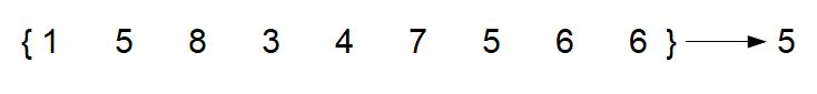
Usually, we compute an average over all our data at once. For example:

It's not a huge stretch to see that we could break this problem into 3 smaller problems and get a very similar result:

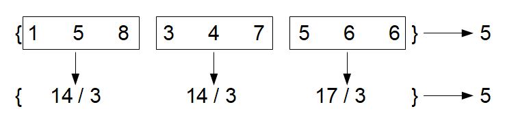
Hopefully the above is quite obvious. Stop for a moment and think about how we could use this... Think about the problem of monitoring a data stream. In a data stream, the flow of data is constant. Over time this will grow to be very large. It's intractable to consider calculating an average over an infinitely growing stream of data. But what we have shown here is powerful: we've been able to calculate the full average from just 3 parts of the data stream. We've just reduced the size of the problem by a factor of 3. This is just the tip of the iceberg though, we can calculate a running average as each data point arrives:

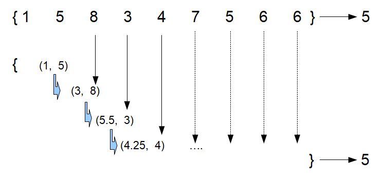
Notice that the problem becomes this nice recursive problem, with no need to store the previous data points. In fact, we can throw away the previous data points and keep just two numbers: the previous "average" and the current data point and take the average at each step:

To me, at least, this is not blindingly obvious. But after playing with a few simple examples I was able to satisfy myself that this was working.

A Real-world Example

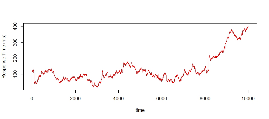
Nothing beats a real-world example. In this example, we are going to track the mean response time for a web service. For simplicity, I've taken a short time slice for this example, 7 days worth of monitoring data where the mean response time has been recorded every 60 seconds. I have also chosen an interesting period, which shows a few ups and downs and a prolonged period of degradation throughout the last day or so. Obviously, this is a small slice of the full dataset, but interesting none-the-less. Here it is:

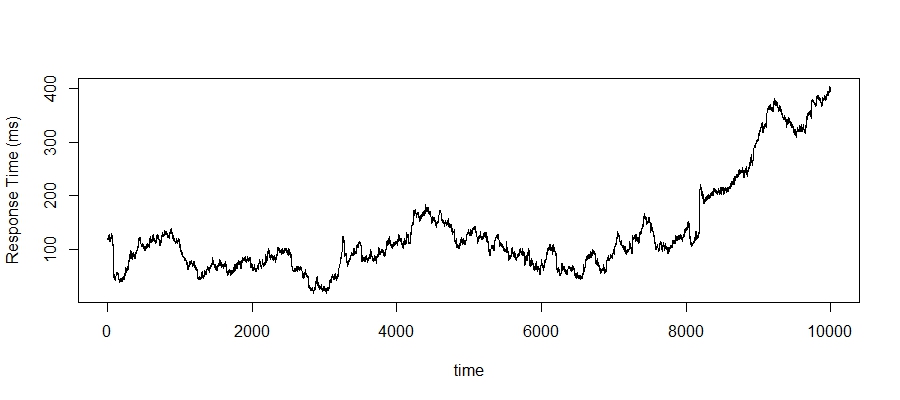
The full dataset is massive now, we've got no hope of being able to do real-time analysis on this using the whole dataset. Along with the size of the dataset, there are other good reasons for using an online average:

1. real-world data is almost always noisy. Excessive noise can seriously skew further analyses and a moving average is quite an effective method for smoothing away the noise
2. real-world monitoring solutions are also plagued by missing data points. An incremental average should be able to smooth through short periods of missing data and thus, allow your downstream analyses to continue
3. any real-world monitoring tool must be adaptable. Hard-thresholds are just not acceptable anymore. Your monitoring systems need to be able to adapt along with the environment they are monitoring.

One of the key statistics we measure is the mean response time over a variety of time windows and this is something I would like to build up to. Let's first start with a simple online moving average (moa). We will create a function in R to calculate this:

moa <- function (x, mu) {
  mu + 0.5*(x - mu)
}

We have essentially, recreated the same time series. It's really hard to see this, but we have actually smoothed the series slightly. There is a black line that is the original series and the red line is the moving average. If you look hard, the red line doesn't quite hit all the peaks of the black line, it is slightly smoother. Why would you want to smooth the series a little? Because we live in a very noisy world and most of the time, we want to reduce the amount of noise whilst not losing the main signal.

We can take this a step further and add additional smoothing to the online average. We achieve this by including a learning rate (alpha), which will further weight the adjustment of the online average:

moa <- function (x, mu, alpha = 0.5) {
  mu + alpha * 0.5 * (x - mu)
}

par(mfrow = c(2, 2)) 
for (i in 0:3) {
  mu <- 0
  z <- apply(matrix(2:10000), 1, function (t) {
    mu <<- moa(iot[t, 1], mu, alpha = 1 / (10 * 2^i))
  })
  plot(iot[, 1], type = "l", col = "darkgrey", main = sprintf("alpha: %s", (0.05 / (10 * 2^i))),
       ylab = "Response Time (ms)", xlab = "time")
  lines(z, col = "red")
}
par(mfrow = c(1, 1))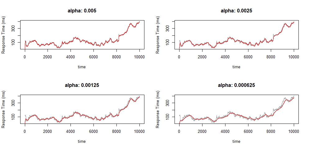

Notice how the online average becomes increasingly smooth. This is a very desirable property because it means that the noise has less influence upon our next layer of analysis. For example, even a large spike, if it is short, will not drastically skew our online average. But as you can see, prolonged periods of degradation are still captured by the online average.

We can have a little more fun with this and exaggerate the distance weighting of the update process. Specifically, if the new data point is close to the online average, then we would like it to have a strong influence on the online update. But if the new data point is a long way away from the online average, we would like to reduce its influence so that our average doesn't swing wildly:

moa <- function (x, mu) {
  mu + (1 / sqrt((x - mu)^2))*(x - mu)
}
mu <- 0
z <- unlist(lapply(2:10000, function (idx) { 
  mu <<- moa(iot[idx, 1], mu)
  return (mu)
}))
plot(iot[, 1], type = 'l', col = 'darkgrey', 
     ylab = "Response Time (ms)", xlab = "time", main = "Distance weighted")
lines(z, col = 'red')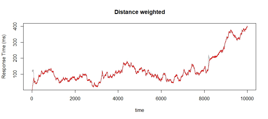

Again, this is tricky to see but look carefully just after time 8000. Notice that the online average doesn't immediately spike along with the true signal. This has become a little too noisy again for my liking, so let's combine the distance weighting along with a learning weight:

moa <- function (x, mu, alpha = 1) {
  mu + (alpha / sqrt((x - mu)^2))*(x - mu)
}
par(mfrow = c(2, 2)) 
for (i in 0:3) {
  mu <- 0
  z <- apply(matrix(2:10000), 1, function (t) {
    mu <<- moa(iot[t, 1], mu, alpha = 1 / 2^i)
  })
  plot(iot[, 1], type = "l", col = "darkgrey", main = sprintf("alpha: %s", (1/2^i)))
  lines(z, col = "red")
}
par(mfrow = c(1, 1))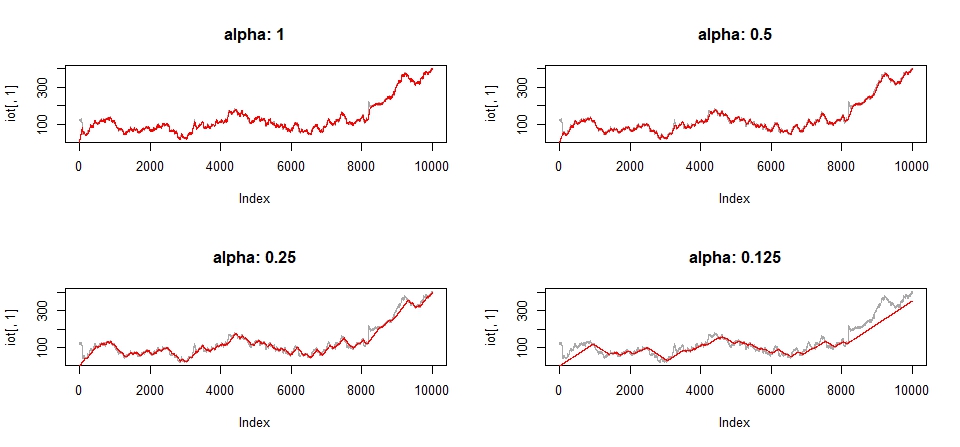

Once again, the online average becomes increasingly smooth as we increase the effect of the learning rate. In fact, you can get some really interesting effects (like the bottom right-hand plot) by increasing the learning rate sufficiently.

Wrap up

It's surprisingly easy to calculate efficient and interesting online averages in real-time data streams. One of the things I like most about these ideas is the amount of fun and customisation you can create by including things like a distance penalty or even just by adjusting the learning rate. We could take these ideas further and use them as the basis of real-time anomaly detection as well. Perhaps we will look at this in the near future.