

Introduction
Sometimes, we need to connect to SQL Server using RStudio, the most common tool for programming in R. R is one of the most popular programming languages for machine learning and data science. In this tutorial, we will teach the following topics:
- I fast hello world example in R.
- How to use variables in R.
- Also, how to check if the R library exists.
- How to connect to SQL Server using RStudio and show data.
- In addition, we will learn how to get statistics from a SQL Server table using RStudio.
- How to install the statistics libraries.
- Advanced statistics measures.
- How to get advanced statistics from a SQL Server table using RStudio.
- How to get charts from a SQL Server table using RStudio.
Requirements
First, we will download R and RStudio from the following links if you do not have them: RStudio and R download page.
Getting started – Hello world example in R
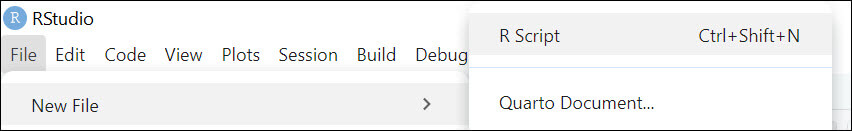
First, we will start the RStudio application.
Secondly, go to the Menu and select File>R Script to run an R script.
Also, use this code:
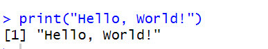
print("Hello, World!")In addition, run the code.
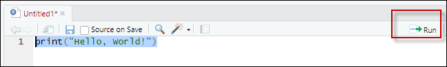
Finally, the code will show a Hello, world message.
Use Variables in RStudio
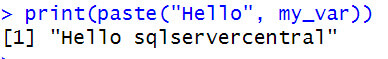
In the next example, we will use variables in RStudio. First, use the following code:
my_var <- "sqlservercentral"

print(paste("Hello", my_var))
Finally, run the code, and you will be able to concatenate the hello with a variable. In this example, the variable stores the sqlservercentral value:
How to check if the R library exists
To connect to SQL Server, we will use the odbc library. This library is commonly used to connect to databases. ODBC (Open Database Connectivity) is a standard API (Application Programming Interface) used to connect databases.
The following code will check if the odbc library is installed. If it is installed, it will display the message that the package is installed. Otherwise, the message will say that the package is not installed.
pkg <- "odbc"

if (requireNamespace(pkg, quietly = TRUE)) {

cat("The '" , pkg , "' package is installed.\n")

} else {

cat("The '" , pkg , "' package is NOT installed.\n")

}
Install the ODBC library in R
If the odbc package is not installed, in the R code, run this code:
install.packages("odbc")The code will install the package.
How to connect to a SQL Server table with RStudio
The following code will connect to SQL Server in RStudio using R. First, we will invoke and use the odbc library. Secondly, we will connect to the SQL Server using the SQL Server Native Client 11.0. To get the list of available drivers, use this code:
library(odbc)

# List all available ODBC drivers

odbcListDrivers()
Thirdly, we will connect to the SQL Server. In this example, we use the localhost, but you can use the SQL Server name.
Also, we are using AdventureWorks2019 in this example. For more information on how to get this database, refer to our sample databases article.
Finally, we are using Windows Authentication (Trusted_Connection = “Yes”) to connect to SQL Server.
The code used is the following:
library(odbc)
# Create the connection to SQL Server

con <- odbc::dbConnect(

odbc::odbc(),

Driver = "SQL Server Native Client 11.0", # or "ODBC Driver 17 for SQL Server"

Server = "localhost", # use the SQL Server name. In this example, we are using the local SQL Server

Database = "AdventureWorks2019", # this is the SQL Server database name

Trusted_Connection = "Yes" # We are using Windows Authentication

)

# Run a query

result <- odbc::dbGetQuery(con, "SELECT * FROM Production.TransactionHistoryArchive")

# View result

head(result)

# Disconnect

odbc::dbDisconnect(con)
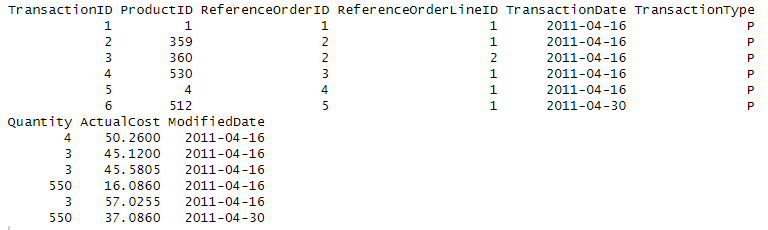
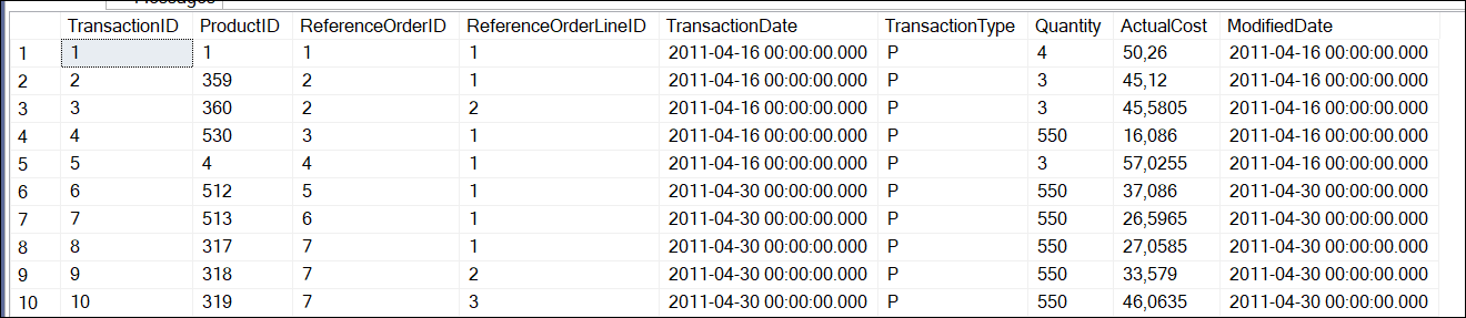
The code will query the information from the Production.TransactionHistoryArchive table. This table belongs to the AdventureWorks2019 table.
The head(result) will display the information. Finally, we are disconnecting with the dbDisconnect function. The information displayed will be the following:
How to get statistics from a SQL Server table using RStudio
Previously, we explained how to get data from SQL Server. Now, we will show some statistics. We will show the maximum value, the minimum, the mean, the median, and the Standard Deviation.
First, we have the Maximum ($Max) and minimum values ($Min). Secondly, we have the Mean and the Median. The mean is the average, which can be calculated by adding up the values and dividing by the number of values. The median is the middle value when the data is ordered from the least to the greatest. Finally, we have the standard deviation ($StdDev) is used to measure the dispersion of a set of data. It shows how much the values deviate from the mean.
We will get information from these 2 columns of our Production.TransactionHistoryArchive:
- Quantity.
- ActualCost.
The code used is the following:
Code in RStudio to get the statistics
library(odbc)

# Create the connection directly

con <- odbc::dbConnect(

odbc::odbc(),

Driver = "SQL Server Native Client 11.0", # or "ODBC Driver 17 for SQL Server"

Server = "localhost",

Database = "AdventureWorks2019",

Trusted_Connection = "Yes"

)

# Run a query

result <- odbc::dbGetQuery(con, "SELECT * FROM Production.TransactionHistoryArchive")

# View first rows

print(head(result))

# Statistics for Quantity

quantity_stats <- list(

Min = min(result$Quantity, na.rm = TRUE),

Max = max(result$Quantity, na.rm = TRUE),

Mean = mean(result$Quantity, na.rm = TRUE),

Median = median(result$Quantity, na.rm = TRUE),

StdDev = sd(result$Quantity, na.rm = TRUE)

)

print("Statistics for Quantity:")

print(quantity_stats)

# Statistics for ActualCost

cost_stats <- list(

Min = min(result$ActualCost, na.rm = TRUE),

Max = max(result$ActualCost, na.rm = TRUE),

Mean = mean(result$ActualCost, na.rm = TRUE),

Median = median(result$ActualCost, na.rm = TRUE),

StdDev = sd(result$ActualCost, na.rm = TRUE)

)

print("Statistics for ActualCost:")

print(cost_stats)

# Disconnect

odbc::dbDisconnect(con)
First, we have the results for Quantity:
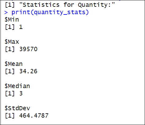
In this case, the maximum quantity is 39570, and the minimum value is 1. The mean is 34.26 and the mean is 3, which means that the quantities are low values. 50 percent of the values will be lower than 3. A Standard deviation of 464 means that data points are spread out from the mean. The quantities vary significantly.
Secondly, we have the results for ActualCost:
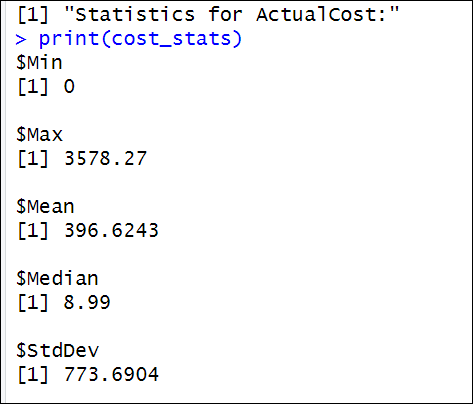
Also, we have the statistics for the actual cost. In this case, the maximum cost is 3578.27, and the minimum value is 0. The mean is 396.6243, and the median is 8.99. This suggests that while the costs tend to be low (with 50 percent of the values below 8.99), the presence of the high maximum cost (3578.27) pulls the average upwards. A standard deviation of 773.6904 indicates that the cost data points are widely spread out from the mean, suggesting significant variability in the costs. The costs vary greatly, with many low values and a few much higher values.
How to install the statistics libraries
Previously, we learn how to get basic statistics. However, R is used for more advanced analysis. For more advanced statistics, we will install the e1071 library and the summarytools library. To do it, run this code:
install.packages("e1071")

install.packages("summarytools")
First, we have the e1071. It is used in statistical models and machine learning in R. It is used for classification and clustering.
Secondly, we have the summarytools. This library is used for data exploration and summarization.
Advanced statistics
In the next section, we will work with the Range, IQR, Variance, Skewness, Kurtosis, Quartiles, Unique values, and Zero count.
Here we will explain each one:
First, we have range. Range is the difference between the maximum and minimum value. It is a simple formula to understand how much the values vary.
Formula: Range=Max−Min
Secondly, the IQR (Interquartile Range). This statistical measure shows the range within which the middle 50 percent of the data falls. The formula is the difference between the 3rd quartile and the first quartile.
Formula: IQR=Q3-Q1.
Thirdly, we have the variance. This number shows how much the values deviate from the mean of the dataset.
Formula:
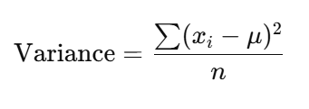
For more information about this formula, refer to this link.
Also, we have the skewness, which shows the asymmetry of the data. If the value is positive, most of the values are small, but a few have higher values. If the skew is negative, most values are big, but there are a few small values high.
Formula:
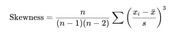
For more information about this formula, refer to this link.
In addition, we have the Kurtosis. This measures the tailedness of the distribution of the data. If kurtosis is close to 3, it means that it has a normal distribution. If the values are higher, there are heavy tails.
Formula:
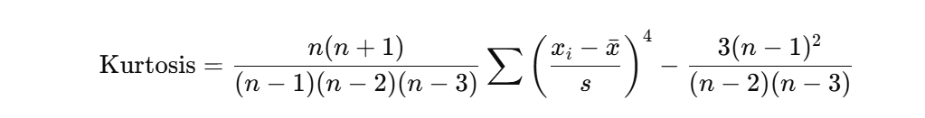
For more information about this formula, refer to this link.
Additionally, we have the quartiles. They are used to divide your data into 4 equal parts. In addition to these measures, we have the unique values to count how many unique values exist. Finally, we have the zero_values function to count the number of values equal to 0.
How to get advanced statistics from a SQL Server table using RStudio.
The following code will connect to the Production.TransactionHistoryArchive table in SQL Server and get statistics like the Range, IQR, Variance, Skewness, Kurtosis, Quartiles, Unique values, and zero count.
library(odbc)

library(e1071) # For skewness and kurtosis

library(summarytools)

# Connect to SQL Server

con <- odbc::dbConnect(

odbc::odbc(),

Driver = "SQL Server Native Client 11.0",

Server = "localhost",

Database = "AdventureWorks2019",

Trusted_Connection = "Yes"

)

# Query the data

result <- odbc::dbGetQuery(con, "SELECT * FROM Production.TransactionHistoryArchive")

# Disconnect

odbc::dbDisconnect(con)

# Filter for numeric columns just in case

quantity <- result$Quantity

cost <- result$ActualCost

# Advanced stats for Quantity

quantity_stats <- list(

Range = diff(range(quantity, na.rm = TRUE)),

IQR = IQR(quantity, na.rm = TRUE),

Variance = var(quantity, na.rm = TRUE),

Skewness = e1071::skewness(quantity, na.rm = TRUE),

Kurtosis = e1071::kurtosis(quantity, na.rm = TRUE),

Quantiles = quantile(quantity, probs = seq(0, 1, 0.25), na.rm = TRUE),

Unique_Values = length(unique(quantity)),

Zero_Count = sum(quantity == 0, na.rm = TRUE)

)

# Advanced stats for ActualCost

cost_stats <- list(

Range = diff(range(cost, na.rm = TRUE)),

IQR = IQR(cost, na.rm = TRUE),

Variance = var(cost, na.rm = TRUE),

Skewness = e1071::skewness(cost, na.rm = TRUE),

Kurtosis = e1071::kurtosis(cost, na.rm = TRUE),

Quantiles = quantile(cost, probs = seq(0, 1, 0.25), na.rm = TRUE),

Unique_Values = length(unique(cost)),

Zero_Count = sum(cost == 0, na.rm = TRUE)

)

print("Advanced statistics for Quantity:")

print(quantity_stats)

print("Advanced statistics for ActualCost:")

print(cost_stats)
The values displayed by the code are the following:
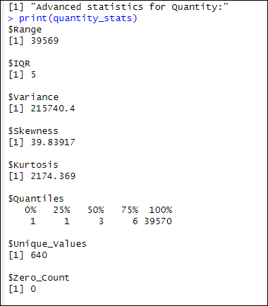
We will explain the values of the Quantity in the next section.
Explanation of the previous results for the Quantity column
Here we will explain the Advanced Statistics from the previous section. First, we have a range of 39569 means that there is a considerable difference between the maximum and minimum value. Also, the IQR = 5 means that most of the data is in a small range of values.
In addition, we have a variance equal to 215740.4, which means that my Quantity values have a high variance, which means that there is a large difference between the Quantity values. Also, the quantity column has a skewness equal to 39.83, which means that the distribution of the data is not symmetric. Additionally, a kurtosis equal to 2174 means that the values have heavy tails.
Also, we have the quartile values.
- First, we have the 0, which contains the Minimum value. This is the minimum value equal to 1.
- Secondly, we have the first quartile. 25 percent of he values in this quartile are less than or equal to 1 for the ActualCost column.
- Thirdly, we have the Q2 quartile with the median. In this quartile, the values are less than or equal to 3.
- Also, we have the Q3 quartile that shows that the values are equal to 6 or lower.
- Finally, the Q4 quartile shows that the maximum value is 39570.
We also have 640 unique values and 0 zeros.
The ActualCost column has the following values:
We will explain the results in the next section.
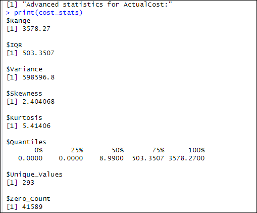
Explanation of the previous results for the ActualCost column
First, we have a range of 3578.27, which means that there is a considerable difference between the maximum and minimum values of the ActualCost data. The range reflects the spread between the smallest and largest cost values in the dataset. Also, the IQR = 503.3507 means that most of the data is in a small range of values, with the middle 50 percent 0f the values falling between the first and third quartiles, which indicates a moderate level of concentration around the middle.
In addition, we have a variance equal to 598596.8, which means that the ActualCost values have a high variance, indicating that the cost values are highly spread out from the mean. This reflects the significant difference between the costs, with some values deviating greatly from the average. Also, the ActualCost column has a skewness of 2.4041, which means that the distribution of the data is not symmetric. Since the skewness is positive, it suggests that the tail of the distribution is pulled to the right, meaning that a few higher-than-usual cost values are impacting the overall distribution.
Additionally, a kurtosis of 5.41406 means that the values have heavy tails. This indicates that there are extreme outliers or unusual values far from the mean, which is typical in datasets with high kurtosis.
We also have the quartile values:
- First, we have the 0, which contains the Minimum value. The minimum value is 0.0000.
- Secondly, we have the first quartile. The values in this quartile are less than or equal to 0.0000 for the ActualCost column.
- Thirdly, we have the Q2 quartile, which is the median. In this quartile, the values are less than or equal to 8.9900.
- The 75 percent quartile shows that the values are equal to 503.3507 or lower.
- Finally, the hundred percent quartile shows that the maximum value is 3578.2700.
We also have 293 unique values and 41589 zeros in the ActualCost column.
How to get charts from a SQL Server table using RStudio
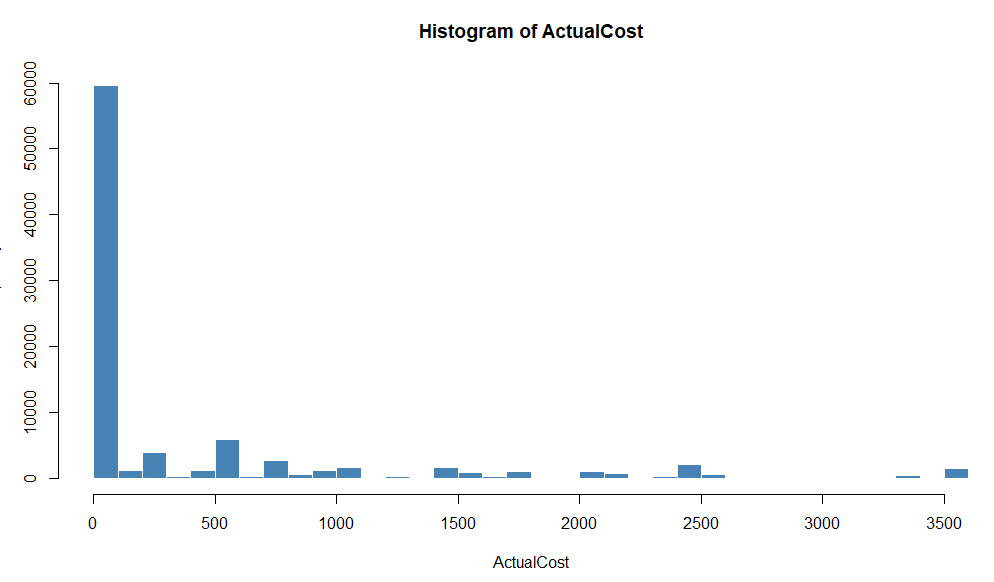
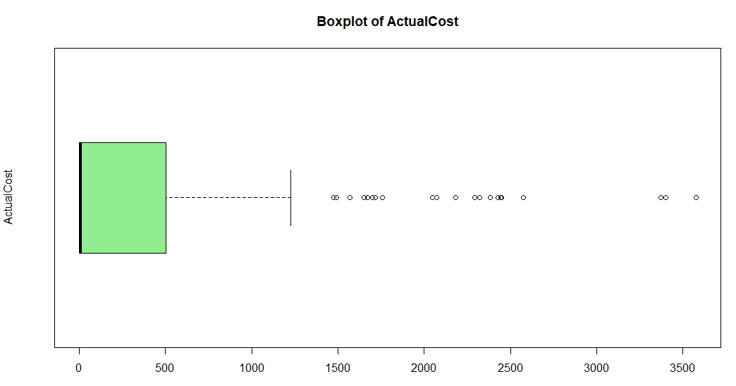
In the last example, we will show how to create a histogram and a boxplot of the data of the actualcost column of the Production.TransactionHistoryArchive table in SQL Server.
The code used is the following:
library(odbc)

# Connect to SQL Server

con <- odbc::dbConnect(

odbc::odbc(),

Driver = "SQL Server Native Client 11.0",

Server = "localhost",

Database = "AdventureWorks2019",

Trusted_Connection = "Yes"

)

# Query the data

result <- odbc::dbGetQuery(con, "SELECT * FROM Production.TransactionHistoryArchive")

# Disconnect

odbc::dbDisconnect(con)

# Extract ActualCost data

actual_cost <- result$ActualCost

# Plot histogram

hist(actual_cost,

main = "Histogram of ActualCost",

xlab = "ActualCost",

col = "steelblue",

border = "white",

breaks = 50)

# Plot boxplot

boxplot(actual_cost,

main = "Boxplot of ActualCost",

ylab = "ActualCost",

col = "lightgreen",
horizontal = TRUE)
The histogram creates a representation of the distribution of your data. It shows the frequency of the data points of your data. As you can see, most of the values are low and close to 0.
On the other hand, we have the Boxplot, which represents your data in distributed in quartiles.
As you can see, most of the ActualCost values are between 0 and 500, and a few values are between 500 to 3500.
Conclusion
In this article, we learned how to connect to SQL Server using R. This is a popular language similar to Python used to analyze data. Also, we learned how to get advanced statistics and create some charts. R is an advanced programming language with a lot of libraries that can provide powerful features to analyze our data in SQL Server.