If you want to be a T-SQL big hitter within your organisation, then stop what you’re doing right now and go to Amazon or Word Press and order a book by Itzik Ben-Gan. I have read many of his books and found they’ve helped me become a much greater SQL Server developer. His work has helped me find many great solutions and the knowledge I’ve gained is the foundation to the article I bring to you today. For those of you that already have a book, release that cherishing cuddle and put the book down. It’s time to get on with some work.

Create sample data

To demonstrate this method to you I will need some sample data. Attached is a script (Article_StrangeG_DBCreate.sql) that will generate some data to work with. The script may take some time to execute, so I suggest start running it now and then continue on reading. The script creates a new database and sets up all the required objects and data in that new database.

I’ve supplied two scripts for populating the database. One will create almost 120 million rows in the Fact table and the second will create around 43 million. I’ve done this to provide options for readers using spinning disks and readers using SSD. The article is based on tests I did on my SSD based system, therefore if you run the 43 million row version you will get different query plans and stats to the ones listed in the article. Below is a table of load times I recorded when testing on other systems.

A more detailed understanding of the sample data is included later in the article. Let’s skip that for now and start looking at how to query this big table.

Querying the Sample Data

I now have a fact table with 120million rows and a bunch of columns with non-uniform distribution, great! Let’s start with something simple and just query the table with some search criteria. If I start by querying one column, product_id. This column is the lead column on a non-clustered index.

I’ll start by querying the table in three different ways to get the same result. Here is the count query with constants.

select count(*)
 from Fact
 where product_id = 1

This query reads 1 row with the parameters provided. The query plan shows that 1 row was estimated so all is well so far.

If I now execute the query again with different parameters, this time returning a large number of rows.

select count(*)
 from Fact
 where product_id = 170

The parameterised plan in cache from the first execution is used and I get dramatically underestimated row counts. If I clean the plan cache and execute again.

sp_recompile Fact;
select count(*)
 from Fact
 where product_id = 170

I get a new parallel plan and very accurate rows estimates. Having a single table query with very inaccurate row count estimates isn’t too bad. However if I’m joining many tables, inaccurate estimates can produce very poor plans. We have observed that querying a table with a large skew in the data distribution can produce widely differing plans and inaccurate estimates depending on which query puts a plan in cache first.

Let’s see what happens when variables are substituted for the constants.

declare @product_id int = 1;
select count(*)
 from Fact
 where product_id = @product_id

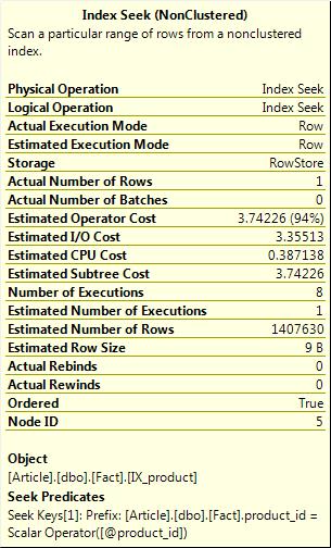
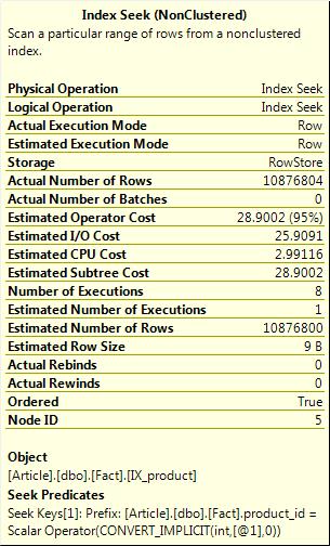
This query produces a plan with an estimate of 1,407,630 rows, huh? Hmm, way more than the single row it actually read. And it produced a parallel plan to read a single row, crazy! Let’s try it again with some parameters that read a lot of rows.

declare @product_id int = 170;
select count(*)
 from Fact
 where product_id = @product_id

Again this query produces a plan with an estimate of 1,407,630 rows. If we recompile the Fact table and run the second query again, the estimate does not change, nor does the plan. So again using this method we observed that querying a table with a large skew in the data distribution can produce widely inaccurate estimates. However, on this occasion we don’t have any difference in plan.

The reasons for the behaviour we observed can be explained with the knowledge of parameterised plan creation and the use of histogram stats vs density estimation. These are vast subjects and outside the scope of this article. So for now we need to simply observe and accept the behaviour.

Now we need to understand how “maybe parameters” affect a query.

Maybe Parameters

To coin the term “maybe parameters” I first need to explain. Typically we express filter criteria as a series of expressions which evaluate against variables and or constants to achieve a Boolean result. We can assume for the most part that filter expressions will create a “definitely filter” and when the expression is evaluated then the result will definitely filter the query output. But this is not always possible and sometimes we want a more dynamic expression.

There are many examples of “maybe parameter” solutions on sites like SQLServerCentral and Stackoverflow, to name a few, and are often described as dynamic or conditional where clauses. Essentially the problem to overcome is ignoring a where condition when no value is supplied to an input parameter of that condition. I prefer the term “maybe parameter” as it’s so much more vague than “optional parameter”. Optional is pleasant and un-concerning, it’s meaning is closely aligned with a Boolean outcome. Maybe is obtuse and indeterminate.

To clarify here are some examples of definitely filters.

SELECT *
 FROM Fact
 WHERE product_id = 1;
SELECT *
 FROM Fact
 WHERE class = @class_id;

Now a “maybe filter” is an expression where a “maybe parameter” is used to filter the result set. Or it does not filter the result if the parameter is un-assigned (NULL). Here are some examples of maybe filters

SELECT *
 FROM Fact
 where (product_id  = @product_id
     OR @product_id IS NULL);
SELECT *
 FROM Fact
 WHERE ISNULL(@product_id, product_id) = product_id;

I’ve also observed the following being used specifically for strings.

SET @search_name = ISNULL(@search_name, ‘%’);
SELECT *
 FROM Fact
 WHERE name LIKE @search_name;

Set let’s try a count query using a maybe parameter

declare @product_id int = 170;
select count(*)
 from Fact
 where (product_id = @product_id or @product_id is null);

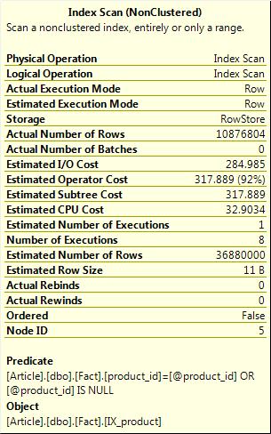
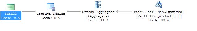
This query produces a plan with an estimate of 36,880,000 rows. The same is true if I try a parameter that filters out just one row. The query also produces an Index scan with a non-sargable predicate and a parallel plans, so even when I wanted just one row from the table I still read 390,641 pages.

set statistics io on;
declare @product_id int = 1;
select count(*)
 from Fact
 where (product_id = @product_id or @product_id is null);

Table 'Fact'. Scan count 9, logical reads 390641, physical reads 0, read-ahead reads 0, lob logical reads 0, lob physical reads 0, lob read-ahead reads 0.

Oh boy, why did SQL Server get it so wrong? Basically we haven’t given it enough clues to build an efficient plan. We’ve basically asked for some of or all of the rows in a 120million table, please. SQL Server just isn’t capable of deriving an efficient plan from this rather vague data request.

What are the alternatives to maybe parameters?

Logic gates: We can use IF statements to first test the input parameters for NULL and act accordingly with multiple implementations of the same query but with different filters. For example, look at this query:

If @product_id IS NULL
BEGIN
       SELECT count(*) FROM Fact
END
ELSE
BEGIN
       SELECT count(*) FROM Fact WHERE product_id = @product_id
END

The problem with this method is that the number of gates required can be expressed with the equation g = p^2 , where g is the number of gates and p is the number of maybe parameters. Therefore if you had a query body that had 20 lines of code and 3 maybe parameters you will end up with 9 logic gates and 180+ lines of code, much of which is repeated. This isn’t the end of the world, but if you imagine this pattern was present in many of the stored procedures in your database then it becomes considerably overweight and code maintenance certainly becomes laboured.

Another alternative

Dynamic SQL (AH, MY EYES!). Why did Microsoft decide to highlight dynamic SQL in red? Psychologically we associate red with danger. So we are already fearful of dynamic SQL through the sub-conscious part of our brain which really doesn’t help.  I have changed my text editor settings to use a mustard colour for string literals, this helps. Syntax highlighting is removed, syntax validation is removed and intellisense is no longer available.

Another problem I have with dynamic SQL is that it breaks the dependency chain. As soon as I start accessing objects in dynamic SQL, I break the dependency chain. Why is this important? Well, a good example of this is when I’m trying to refactor code and I want to know about all the code instances where a table is being accessed.

However dynamic SQL is certainly a good option here. The requirement is to query a table in a very dynamic manner, so why not use dynamic code? I’ve certainly seen many successful implementations of dynamic SQL. On the down side, text manipulation in T-SQL can be cumbersome when compared with other languages like .NET. We also end up with a fairly fragmented routine of code that builds the query up piece by piece. Not the end of the world but still cumbersome and it lacks the elegance of a well written query.

Alternative Three

Use a query engine written in .NE or Java. Again not a bad option here due to the dynamic nature of the requirement. And again I’ve seen many successful implementations of T-SQL query engines. However the trouble you run into here is that the database code gets generated by a bunch of guys and girls that have intermediate T-SQL knowledge and therefore we end up with underperforming code (in my experience). Plus this is an article for DB guys and girls so let’s forget about .NET and Java for now.

The little known wonders of TVF (Table-Valued Functions)

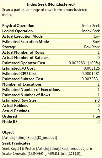
Mr Ben-Gan tells us about the wonders of TVF is his books and a special property they pose. When a constant is passed to a TVF as a parameter, the parameter is parsed into the query as a constant and is not replaced with any parameterisation attempt by the optimizer. We can see an example of this by executing the following TVF SimpleSeek that counts the rows in the Fact tables filtered by 3 Maybe Parameters.

create function [dbo].[SimpleSeek](@product_id int = null, @class_id int = null, @date_id int = null)
returns table
as
return
       select count(*) rc 
       from Fact f
       where (@product_id = product_id or @product_id is null)
       and
       (class_id = @class_id or @class_id is null)
       and
       (f.date_id = @date_id or @date_id is null);

NOTE: Throughout the article I will include the create object statements to assist the narrative. However there is no need to run the code as its already present in the accompanying setup scripts.

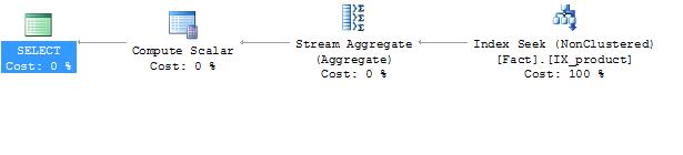
Executed statically, we have

select *
 from SimpleSeek(170,1,1);

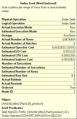
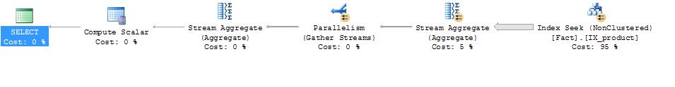
Executed with variables, this is

declare @product_id int = 170, @class_id int = 1, @date_id int = 1;
select *
 from SimpleSeek(@product_id, @class_id, @date_id);

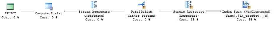
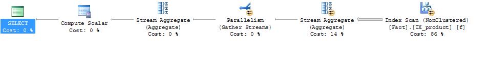
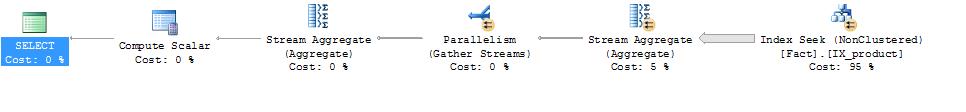
The first query produces a beautifully efficient plan making excellent use of the covering index. It read 17 pages to complete the query. The second query when executed scales-out to a parallel plan because of the substantial load, all because we passed variables into the TVF.

What happens if we force a serial execution of the second query for comparison of the two queries executed on the same amount of processing resources?

declare @product_id int = 170, @class_id int = 3, @date_id int = 1;
select *
 from SimpleSeek(@product_id, @class_id, @date_id)
 option (MAXDOP 1);

Table 'Fact'. Scan count 9, logical reads 390271, physical reads 0, read-ahead reads 0, lob logical reads 0, lob physical reads 0, lob read-ahead reads 0.

The first query took an un-traceable amount of time 0ms and the second query took 2368ms, to read 386114 pages, ouch! 

So the first query’s performance is considerably superior in terms of speed and resource consumption. Plus the solution, as it stands, maintains the dependency chain. However in its current form its static and I can’t supply my maybe parameter values as variables.

I can fix that easily with a call to sp_excutesql right? Lets try…

declare @product_id int = 170, @class_id int = 1, @date_id int = 1;
exec sp_executesql N'select * from SimpleSeek(@product_id, @class_id, @date_id)', N'@product_id int, @class_id int, @date_id int',
       @product_id = @product_id,
       @class_id = @class_id,
       @date_id = @date_id;

I get…

Hey! What happened to my nice efficient plan! It would seem that the sp_executesql sp stripped away the TVF magic. Of course it did. If you look closely at the cmd string I’m still passing parameters into the TVF and not constants. Of course I am, sp_executesql is our SQL Injection protection protocol. OK, I can fix that, by making a classic dynamic SQL call.

declare @product_id int = 170, @class_id int = 1, @date_id int = 1;
declare @cmd nvarchar(4000) = (N'select * from SimpleSeek('
       + cast(@product_id as nvarchar(12)) + ','
       + cast(@class_id as nvarchar(12)) + ','
       + cast(@date_id as nvarchar(12)) + ')');
exec (@cmd);

I get…

Great! My efficient plan is back. However my code is now looking a bit ugly. And am I introducing SQL Injection risk? No, I can’t inject SQL into the call to a TVF, because the TVF contains declared code not dynamic code.  However if I needed to start passing in string parameters then I am indeed open to SQL Injection.

Is there an alternative to the dynamic SQL method? Yes, I can use the option (recompile) hint…

declare @product_id int = 170, @class_id int = 1, @date_id int = 1;
select *
 from SimpleSeek(@product_id, @class_id, @date_id)
 option (recompile);

Using this option means that I can encapsulate the structure of the query in the TVF and remove the need to invoke dynamic SQL. I do this because we’re writing a method that will efficiently operate with highly volatile parameter values. So we don’t expect there to be a limited set or a single plan that will be sufficient. So we’re committing to compile time with every execution, but that’s OK. We know we have a big table to process so the compile trade off will be worth it.

The query produced…

Table 'Fact'. Scan count 1, logical reads 17, physical reads 0, read-ahead reads 0, lob logical reads 0, lob physical reads 0, lob read-ahead reads 0.

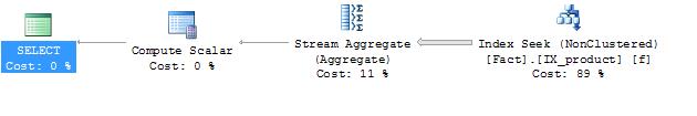
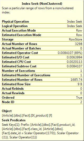
Wow, I’m back to a really efficient plan, fairly accurate row statistics and the query only needed to read 17 pages of data. I’m very happy.

So what happens when I query the table using a predicate that isn’t the lead column in any available indexes?

declare @product_id int =null, @class_id int = 1, @date_id int = null;
select *
 from SimpleSeek(@product_id, @class_id, @date_id)
 option (recompile);

Alas this is where the fanfare stops. Because the class_id column is not the lead column in any available index the SQL optimiser has to make a full or partial scan of an available index with a non-sargable predicate. So although this method of querying creates super-efficient plans the query optimizer can only exploit the available indexes to get super-fast query times.

Dependency Chain

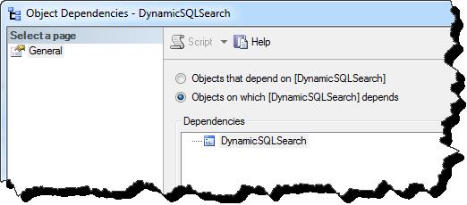
To illustrate the broken dependency chain when dynamic SQL is used as opposed to the TVF method I’ve included two screen shots from SSMS. In the sample database Article_StrangeG there is a stored procedure that wraps up the Dynamic SQL code we reviewed earlier.  As you can see the dependency chain is broken.

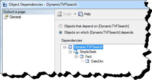
I have a second stored procedure that wraps up the method using the TVF with option recompile hint. As you can see the dependency chain is maintained.

Statistics

Throughout the article I’ve mentioned the importance of accurate statistics but haven’t alluded to any significant advantage of accurate statistics. I imagine many SQL developers have run into a scenario where a stored procedure was executing fine for months and then all of a sudden the performance fell off a cliff. Why? A lot of the time it’s because a bad query plan was created and cached. And the main reason for bad plans? Inaccurate statistics. Using the recompile hint means that the plans produced aren’t cached so there is no chance of pulling a bad plan from cache.

Multiple tables

Let’s see what happens when multiple tables are involved. By adding a join to the DateDim I can start filtering my data by year.

CREATE function [dbo].[YearJoinSeek](@product_id int = null, @class_id int = null, @date_id int = null, @year_id int = null)
returns table
as
return
       select count(*) rc
       from Fact f
       inner join DateDim d
              on f.date_id = d.Date_Id
       where
       (@product_id = product_id or @product_id is null)
       and
       (class_id = @class_id or @class_id is null)
       and
       (f.date_id = @date_id or @date_id is null)
       and
       (d.DateYear = @year_id or @year_id is null);
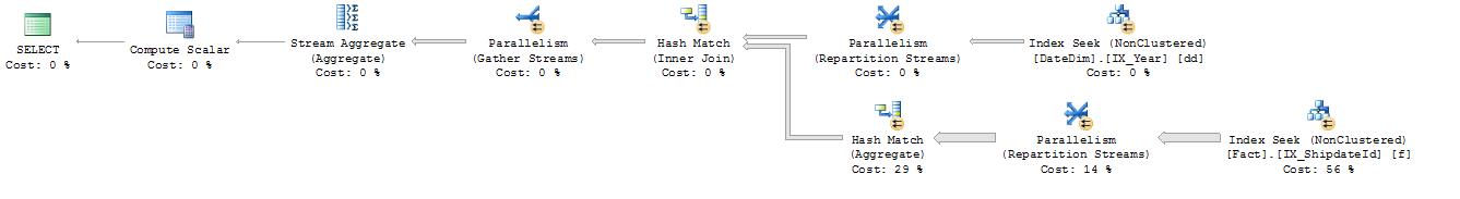
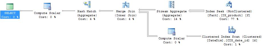
GO

declare @product_id int = 170, @class_id int = 1, @date_id int = null, @year_id int = 2011;
select *
 from YearJoinSeek(@product_id, @class_id, @date_id, @year_id)
 option (recompile);

Table 'DateDim'. Scan count 1, logical reads 4, physical reads 0, read-ahead reads 2, lob logical reads 0, lob physical reads 0, lob read-ahead reads 0.

Table 'Fact'. Scan count 1, logical reads 8807, physical reads 0, read-ahead reads 0, lob logical reads 0, lob physical reads 0, lob read-ahead reads 0.

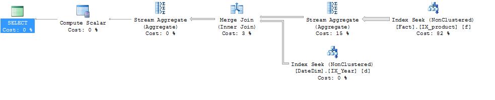
When executed with a year filter I get an efficient merge join and 8807 page reads. So what happens if I don’t supply a year parameter. Do I still need to visit the DateDim table? Conceptually, no. By not supplying a year value I’m inferring that I don’t want to filter by any date. However, logically the answer is yes. My “inner join” states not only that I might filter by year but it also states that all my Fact.date_id values should exist in the DateDim table. So can I avoid making a lookup to the datedim table even if I exclude the condition in the where filter?

I execute the following to find out…

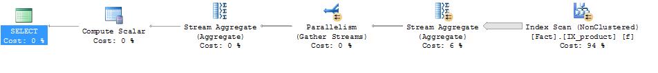
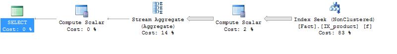
declare @product_id int = 170, @class_id int = 1, @date_id int = null, @year_id int = null;
select *
 from YearJoinSeek(@product_id, @class_id, @date_id, @year_id)
 option (recompile);

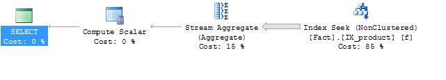
Wow, I didn’t need to visit the DateDim table at all, why is this? The answer is very simple; I have a foreign key between the Fact and DateDim tables that tells the query optimiser that all the Fact.date_id values must exist in the DateDim table. Great! I get a nice efficient plan for my year_id “maybe parameter”. Not having to visit dimensions can be a really significant gain when multiple dimensions are referenced and when you consider a product dimension for a supermarket chain, which may contain millions of rows.

However if the foreign key is created with “NOCHECK” or “NOT FOR REPLICATION” (essentially untrusted), the data cannot be considered consistent by the optimizer. Therefore the DateDim table would still be accessed. Moreover on some occasions you may need to reference a table that doesn’t have a foreign relationship. In these circumstances you can reform your query to avoid the accessing a table unnecessarily.

CREATE function [dbo].[YearJoinExistsSeek](@product_id int = null, @class_id int = null, @date_id int = null, @year_id int = null)
returns table
as
return
       select count(*) rc
       from Fact f
       where
       (@product_id = product_id or @product_id is null)
       and
       (class_id = @class_id or @class_id is null)
       and
       (f.date_id = @date_id or @date_id is null)
       and
       (@year_id is null or exists(select 1 from DateDim dd where dd.Date_Id = f.date_id and dd.DateYear = @year_id));

The two queries below produce exactly the same query plan.

declare @product_id int = 170, @class_id int = null, @date_id int = null, @year_id int = 2011;
select *
 from YearJoinSeek(@product_id, @class_id, @date_id, @year_id)
 option (recompile);

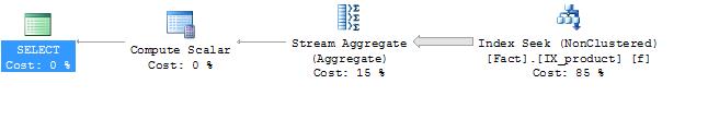
declare @product_id int = 170, @class_id int = null, @date_id int = null, @year_id int = 2011;
select *
 from YearJoinExistsSeek(@product_id, @class_id, @date_id, @year_id)
  option (recompile);

If I omit the @year_id filter and remove the foreign key between fact and datedim table, the second query optimizes to remove the unnecessary access to datedim but the first query does not.

declare @product_id int = 170, @class_id int = null, @date_id int = null, @year_id int = null;
select *
 from YearJoinSeek(@product_id, @class_id, @date_id, @year_id)
 option (recompile);

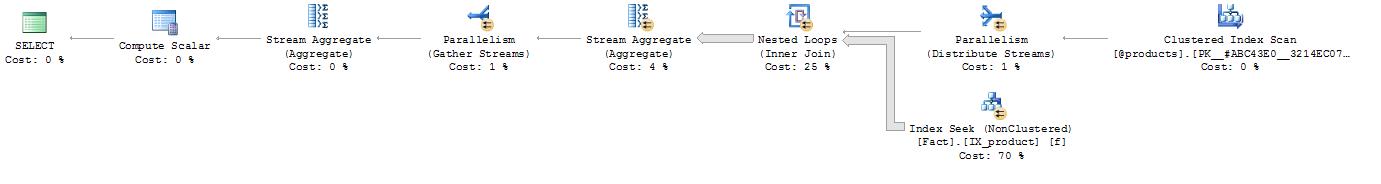
declare @product_id int = 170, @class_id int = null, @date_id int = null, @year_id int = null;
select *
 from YearJoinExistsSeek(@product_id, @class_id, @date_id, @year_id)
 option (recompile);

In this scenario you can even omit the option (recompile) hint and the SQL Server optimizer does have a trick up its sleeve. It adds a startup expression and a Filter plan-operator to try and optimize the work load. However in this specific scenario this has a reverse affect and actually makes for a very poorly performing plan. With multiple scans of the Fact table.

declare @product_id int = 170, @class_id int = null, @date_id int = null, @year_id int = 2011;
select *
 from YearJoinExistsSeek(@product_id, @class_id, @date_id, @year_id);

Table 'Fact'. Scan count 489, logical reads 193410, physical reads 20, read-ahead reads 619, lob logical reads 0, lob physical reads 0, lob read-ahead reads 0.

Table 'DateDim'. Scan count 9, logical reads 4, physical reads 0, read-ahead reads 7, lob logical reads 0, lob physical reads 0, lob read-ahead reads 0.

Table 'Worktable'. Scan count 0, logical reads 0, physical reads 0, read-ahead reads 0, lob logical reads 0, lob physical reads 0, lob read-ahead reads 0.

Table 'Worktable'. Scan count 0, logical reads 0, physical reads 0, read-ahead reads 0, lob logical reads 0, lob physical reads 0, lob read-ahead reads 0.

Multiple Values per Parameter.

What happens if I want to query the data by selecting multiple product ids? If I was writing the query freehand it might look something like the following…

SELECT COUNT(*)
 FROM Fact
 WHERE product_id = 170 or product_id = 169;

What’s very clear from the syntax is that the only way to make this query dynamic is to use dynamic SQL. Sure I could build up multiple parameters calling them @product_id1, @product_id2, etc. And put them all in maybe filters with option (recompile) and it would work. But what about the scenario when the number of product_id’s requested is dynamic. This method won't work anymore, I need something more dynamic. I can do this by adding a TVP maybe parameter.

For example…

CREATE function MultiProductSeek(@product_id int = null, @class_id int = null, @date_id int = null, @multiProducts bit = 0, @products SystemCore.uddt_ids readonly)
returns table
as
return
       select count(*) rc from Fact f
       where
       ((@product_id = product_id and @multiProducts = 0) or @product_id is null)
       and
       (class_id = @class_id or @class_id is null)
       and
       (f.date_id = @date_id or @date_id is null)
       and
       ((@multiProducts = 1 and exists(select 1 from @products p where p.Id = f.product_id) ) or @multiProducts = 0);
GO

I can now execute this function with 3 possible product_id criteria. First with no product filter.

declare @products SystemCore.uddt_Ids;
declare @product_id int = null, @class_id int = 1, @date_id int = null, @multiProducts bit = 0;
select * 
 from MultiProductSeek(@product_id, @class_id, @date_id, @multiProducts, @products)
 option (recompile);

Now with a single product filter…

declare @products SystemCore.uddt_Ids;
declare @product_id int = 170, @class_id int = 1, @date_id int = null, @multiProducts bit = 0;
select *
 from MultiProductSeek(@product_id, @class_id, @date_id, @multiProducts, @products)
 option (recompile);

And multiple product filters…

declare @products SystemCore.uddt_Ids;
insert into @products values (170), (169);
declare @product_id int = null, @class_id int = 1, @date_id int = null, @multiProducts bit = 1;
select *
 from MultiProductSeek(@product_id, @class_id, @date_id, @multiProducts, @products)
 option (recompile);

Table '#ADAC8680'. Scan count 1, logical reads 2, physical reads 0, read-ahead reads 0, lob logical reads 0, lob physical reads 0, lob read-ahead reads 0.

Table 'Worktable'. Scan count 0, logical reads 0, physical reads 0, read-ahead reads 0, lob logical reads 0, lob physical reads 0, lob read-ahead reads 0.

Table 'Fact'. Scan count 2, logical reads 22369, physical reads 0, read-ahead reads 0, lob logical reads 0, lob physical reads 0, lob read-ahead reads 0.

Table 'Worktable'. Scan count 0, logical reads 0, physical reads 0, read-ahead reads 0, lob logical reads 0, lob physical reads 0, lob read-ahead reads 0.

The no-product filter and single product filter executions provide very efficient plans as expected and pages reads are minimal. The multiple product filter execution produces a fairly efficient plan but it’s not as good as using static SQL or therefore using dynamic SQL. Here is a static SQL example:

declare @product_id1 int = 170, @product_id2 int = 169, @class_id int = 1;
SELECT COUNT(*)
 FROM Fact where
(
    (@product_id1 = product_id or @product_id2 = product_id )
    or
    COALESCE( @product_id1, @product_id2 ) IS NULL
)
and
(class_id = @class_id or @class_id is null)
 option (recompile);

Table 'Fact'. Scan count 15, logical reads 20111, physical reads 0, read-ahead reads 0, lob logical reads 0, lob physical reads 0, lob read-ahead reads 0.

Although it’s not as efficient as the dynamic SQL option, it’s still a choice worth considering as it produces a good plan, page reads are comparable to the static/dynamic SQL option, the code is cleaner and the dependency chain is maintained.

Dynamic, Efficient Group by

Often a report will need data grouped by attributes. At first it may not be obvious that a group by clause can be dynamic, however this isn’t entirely true. We have some flexibility when the case statement is introduced.

I’ve prepared an example of how this works.

CREATE function YearJoinGroupSeek(@product_id int = null, @class_id int = null, @date_id int = null, @year_id int = null, @group_by sysname = null)
returns table
as
return
       select case when @group_by = 'DateMonth' then d.DateMonth else -1 end grp, count(*) rc
       from Fact f
       inner join DateDim d
              on f.date_id = d.Date_Id
       where
       (@product_id = product_id or @product_id is null)
       and
       (class_id = @class_id or @class_id is null)
       and
       (f.date_id = @date_id or @date_id is null)
       and
       (d.DateYear = @year_id or @year_id is null)
       group by case when @group_by = 'DateMonth' then d.DateMonth else -1 end;
go

Using this method of customizing the group by clause in conjunction with the option recompile hint means that a re-grouping of the data can be dynamic and the plan that’s produced also dynamic and efficient.

Here are some examples of how the execution for grouped and un-grouped calls to the function YearJoinGroupSeek play out.

declare @product_id int = 170, @class_id int = 1, @date_id int = null, @group_by sysname = 'DateMonth';
select *
 from YearJoinGroupSeek(@product_id,@class_id,null,null, @group_by)
 option ( recompile );

declare @product_id int = 170, @class_id int = 1, @date_id int = null, @group_by sysname = null;
select * 
 from YearJoinGroupSeek(@product_id,@class_id,null,null, @group_by)
 option ( recompile );

As you can see again we get very efficient plans for both function calls. Having this type of query does however mean the second call ends up with a redundant column. This seems to be a small price to pay for a neat, efficient, dynamic pattern.

Sample Data

So what does our dummy data need to look like? Well, I need a table with a lot of rows, a bunch of columns and a distribution that isn’t uniform. Why? Because most columns of data do not have uniform distribution. To create non-uniform distribution I’m going to create a column using the formula y = 1.1^x to get a steep skew in the data clusters. You may want to bring the accompanying script code up in SSMS as you go through this section.

Table schema

Date_id int, with a data distribution approximately equal to the equation y = √ 1.1^x

Shipdate_id int, with a data distribution approximately equal to the equation y = √ 1.1^x

class_id int, with a data distribution that is uniform with 3 values

product_id int, with a data distribution approximately equal to the equation y =  1.1^x

A clustered key exists on the date_id column as date intervals are a typical filter criteria within any organisation.

Creating non-uniform distribution

To demonstrate non-uniform data distribution:

Uniform data distribution

1,2,3,4,5,6,7,8,9,10,11,12,13,14,15

Non-uniform distribution

1,2,3,4,4,5,5,5,5,5,6,6,6,6,6,6,6,6,6,6,6,6,6,6,6,6

I’m sure there are more mathematically complex ways of producing non-uniform data, but this method will suffice for demo purposes. The formula x = 1.1^y is just a guide rope for the distribution and I will use a derivative of the graph to produce the row counts which allows me to construct a table in a more efficient fashion. I’ll describe how I arrived at this formula later.

To materialise large amounts of data from none I will need a tally table.  To create a tally table I will use a small virtual tally table to generate the materialised tally table rows. By generating 10 virtual rows I can cross join this table twice to produce my Tally table with rows = 10^3. Put an index on the tally table and I’m done.

My next challenge is to create the non-uniform distribution that I referred to previously. So I know the graph x = c^y will produce a nice bell curve, but how do I arrive at c? Well I know I want to make a lot of rows, so 100million rows would be a good target and I’d like my biggest cluster of rows to be roughly 10% of the target row size. So I could work this out using some maths, but instead I tried a few trial and error iterations changing c and quickly arrived at 1.1. Using this constant gives me total rows 119715152.3 and a maximum cluster size of 10883196.7. So I over shot the total row size by 20%, but I’m happy with that, its close enough. Using the formula I can achieve the desired target row count in 170 iterations of y.

Now I have an understanding of the shape of the data that I’m going to create, I’m going to store this information in an intermediate table called steps.

To generate the actual rows I use the square root of the cluster size to build a sub-table that when cross joined will produce the target number of rows. By storing the square root in the steps table I no longer need to store the target cluster size, but I will keep in there for demonstration purposes. I also keep the step number in as it will become the data values for the data clusters.

Conclusion

The methods I’ve described in the article address many of problems encountered when developing queries that have dynamic requirements. I believe the methods promote efficient and maintainable code, that’s hopefully easier on the eye and maintains the dependency chain. Hopefully I’ve given you the knowledge that will help you create queries that will run efficiently when your data starts to get really big. The methods I’ve written about are still applicable to smaller tables but you have to weigh up whether forced recompilation (option (recompile)) is appropriate for a given work load. I really hope you've enjoyed reading this article and its contributed to your understanding of how to get the most out of SQL Server.