Introduction

As database professionals we all probably at some point had to deal with some kind of data monitoring. It could be system data from the very servers we manage or business operational data. And the main purpose of such monitoring usually is to answer one seemingly simple question – if the data shows the signs of being abnormal. The standard approach to tackle this is to have a baseline for the metric you are concerned with and compare the current value with the baseline.

That could be a really challenging task. Just imagine that your data has a high seasonality (low months vs. holiday season) or changes greatly between night and day hours. You might end up with collecting your baseline data hourly for an entire year. To make it worse - once the baseline is established you need to decide how much deviation is too much. In other words, passing what threshold is enough to warrant an alarm? You don’t want to be woken up in the middle of the night just to learn that nothing special is going on with your system; in that case you just set your threshold too low. Nor do you want to learn someday that your system has not worked as expected for a while but you were not aware, as you set your threshold too high.

So is there any other way? Can data itself give us a hint that something is going on, without baselines and thresholds? The answer is yes – if we use a statistical approach and let the data speak. In order to do so we will need...

A Bit of a Theory

The best approach would be to judge the observed value based on its probability, as it’s much easier to deal with probabilities rather than the absolute values themselves. With probability one always can tell that the probability of 0.1% is indeed low and the probability of 99.9% is high. No questions here. Compare this to the case when you only know that your observed value differs from your average by 25%. This could mean anything: no issue at all if your data is highly dispersed and possibly critical situation if your data is very homogeneous.

To figure out what the probability is of seeing the observed value, we need to know the probability density function for your data. Simple. Well, not exactly. The function is known only for a few distributions, of which the Normal is the most widely used. If your data is distributed normally (or close enough), you can calculate probability for your observed value either by using the analytical probability density function or by looking through pre-calculated values in special tables.

For instance, to find out the value with the probability of 0.15% or less you just need to calculate the average value and the standard deviation of your data set (the functions are usually built-in in many program languages, including T-SQL). Once you know the average and the deviation it’s easy to find the value: AVG-3*STDEV (a well-known 68-95-99.7 rule). The rule refers to the both ends of the distribution and you are interested in only one, (either low or high values), thus you take only a half of the value. The problem though that there is a good chance that your data is not distributed normally.

Though you still can work from an assumption of normality I would like to introduce another approach. We can build our probability density function (table valued of course, not analytical) out of data at hand and use it in the exactly same way as one for the Normal Distribution to calculate probabilities. So what is a probability density function?

As complicated as it sounds it’s actually a data histogram on steroids. Imaging that you measure some characteristic of your system periodically. The value of each individual measure becomes a data point in your dataset (called time series). And a histogram simply displays how many of your data points fall to specific range of values you measured. That is shows a dependency of the quantities of data points (Axis Y) from measured values (Axis X).

To build a histogram we need to estimate a bin size (we will use Freedman-Diaconis rule as a guidance) and “pour” the data into the bins. More details can be found in the attached code. Once the histogram is completed we need to normalize the quantities inside the every bin by total number of data points in your data set. And the last step in converting your histogram to a probability density function is to divide normalized quantities by their respective value ranges (like “spreading” them over Axis X).

One can say – OK, I have the function but what about the probability? The probability is the area under the curve. That is to find the probability to see a value equal or greater than V, we need to find the area under the curve from V (on Axis X) to the very end (the right end) of the curve.

Now that we know how to go about it, we can get started.

The Problem

Imagine that you have a server (or more likely a farm of servers) where users upload their files. We have a table where each record represents one upload with a start time, an end time, a file size and maybe a status with success or failure. We would like, from the data alone, to be able to tell if our system is healthy or if there is trouble brewing.

One really important thing here is to choose a proper metric. Though a few can be employed, we will use a ratio of uncompleted uploads in a period of time to the total number of uploads in the same period. We just need to make sure that the chosen interval is such that the substantial number of uploads normally get finished within it so the ratio is not too close to 1. Usually about a half should suffice.

Due to the natural limitations of the selected metric (it’s always between 0 and 1), the values will not be distributed normally, but nevertheless the distribution likely will resemble the normal one (well up to some degree of course). The figures below represent an example of a real probability density function where the time interval was chosen to have about half of uploads completed for Figure 1 and ~70% for Figure 2 (it should be mentioned that the data was collected at different times).

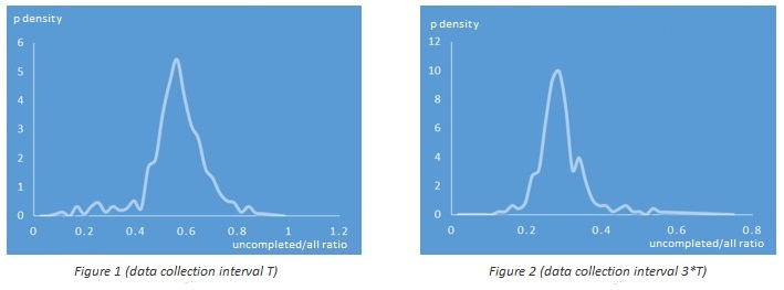
You can see that the probability density function on Figure 1 is quite similar to the one of the Normal Distribution and the function on Figure 2 is noticeably different (due to the longer right tail). And indeed if you calculate the threshold value for the probability 0.15% using the Normal Distribution and this article approach for Figure 1 dataset you won’t find any significant difference while for Figure 2 dataset the difference will be quite noticeable.

Bits and pieces

OK, let’s start coding! First of all as we will put all our objects to a schema called monitor we need to create it.

create schema monitor
go

Next we will create a couple of new types that we will be using to represent our dataset:

create type monitor.timeseries as table(value float)
go

and our probability density table function:

create type monitor.pfunction as table(right_boundary float, cumulative_probability float, id int)
go

Now the core procedure that generates the probability density function:

create procedure [monitor].[get_pfunction]
 @timeseries monitor.timeseries readonly
as
/*
  Generates cumulative probablity table function
  Returns table of type monitor.pfunction
  
  Note that cumulative probability function is descending from 1 to 0. 
*/set nocount on
declare @t table(value float, id int identity(1,1))
insert @t(value) 
select value from @timeseries order by 1
declare @bw float, @min float, @max float, @n float
select @n = count(*), @max = max(value), @min = min(value) from @t
-- finding initial bin size
declare @iqr float, @n1 float, @n3 float, @q1 float, @q3 float, @f1 float, @f2 float, @nb int
set @n1 = (@n +1)/4.00
set @n3 = 3*(@n +1)/4.00
if( @n1 != ceiling(@n1) )
begin
    select @f1 = value from @t where id = floor(@n1)
    select @f2 = value from @t where id = ceiling(@n1)
    set @q1 = (@f1+@f2)/2
end
else
    select @q1 = value from @t where id = @n1
if( @n3 != ceiling(@n3) )
begin
    select @f1 = value from @t where id = floor(@n3)
    select @f2 = value from @t where id = ceiling(@n3)
    set @q3 = (@f1+@f2)/2
end
else
    select @q3 = value from @t where id = @n3
-- this is interquartile value
set @iqr = @q3-@q1 
-- using Freedman-Diaconis rule as a "guidance" to calculate initial bin size:
set @bw = 2*@iqr*power(cast(@n as float), -1/3.00)
-- if bin width is zero (which is a rare case) will use some rather arbitrary number
if( @bw = 0 ) set @bw = 2*sqrt(@n)
declare @x table(f float, bw float, id int identity(1,1))
declare @h1 table(bw float, id int identity(1,1) primary key)
declare @h2 table(rb float, id int identity(1,1) primary key)
declare @hst table(rb float, frequency int, id int identity(1,1) primary key)
declare @hist table(rb float, frequency int, density float, old_density float, id int identity(1,1) primary key)
declare @tp table(rb float, density float, cumulativeProb float, rba float, id int identity(1,1) primary key)
set @nb = ceiling((@max-@min)/@bw)
-- we are using variable bin size (proportional to value) if otherwise we have nonsensical number of bins
if( @nb > @n/3 /*to keep # of bins reasonably low - rather arbitrary*/ )
begin
    insert @x(f, bw)
    select case when value/@bw > 1 then ceiling(value/@bw) else 1 end, case when value/@bw > 1 then ceiling(value/@bw) *@bw else @bw end 
      from @t 
    order by value
    insert @h1(bw)
    select distinct bw from @x order by bw
end
else
begin
    insert @h1(bw) select top(cast(ceiling(@max/@bw) as int)) @bw from @t
end
declare @id int, @idmax int, @rb float = 0
select @id = min(id), @idmax = max(id) from @h1
while @id <= @idmax
begin
    select @rb = @rb +bw from @h1 where id = @id
    insert @h2(rb) values(@rb)
    set @id = @id +1
    if( @rb>@max) break
end
-- histogramm table
insert @hst(rb, frequency)
select h.rb, sum(case when t.value is not null then 1 else 0 end) 
  from @h2 h
       left join @h2 hp on hp.id = h.id-1
       left join @t t on h.rb >= t.value and (hp.id is null or hp.rb < t.value)
group by h.rb
order by 1
-- p density table
insert @hist(rb, frequency, density)
select h1.rb, h1.frequency, h1.frequency/@n/(h1.rb-isnull(h2.rb, 0))
  from @hst h1
       left join @hst h2 on h2.id = h1.id-1
order by h1.id
-- approximate "tail" to the right
declare @pd float, @x0 float
select @pd = density from @hist where id = (select max(id) from @hist)
select top 1 @id = id from @hist where density > @pd order by id desc
-- linear regression (y = ax +b)
declare @xa float, @ya float, @a float, @b float
select @xa = avg(rb), @ya = avg(density) from @hist where id >= @id
select @a = sum((rb-@xa)*(density-@ya))/sum(power((rb-@xa),2)) from @hist where id >= @id 
set @b = @ya -@a*@xa
-- this will be the last point where p density = 0
set @x0 = -@b/@a 
select @idmax = max(id) from @hist 
-- adjust previous points p density according to regression (so that total probablity = 1)
while @id <= @idmax
begin
    update @hist set density = @a*rb +@b, old_density = density where id = @id
    set @id = @id +1
end
-- now we need to adjust density due to increased length
declare @mrb float
select @mrb = rb from @hist where id = @idmax
if( @x0 > @mrb )
begin
    declare @dx float
    set @dx = @mrb -(select rb from @hist where id = @idmax-1)
    update @hist set density = density*@dx/(@x0 -@mrb) where id = @idmax
end
delete from @hist where rb > @x0
insert @hist(rb, density) values(@x0, 0)
insert @tp(rb, density) 
select rb, density from @hist order by id
-- calculate cumulative probability
declare @cp float, @idmin int
select @idmin = min(id), @idmax = max(id) from @tp
set @id = @idmax
while @id > @idmin
begin
    select @cp = sum((h1.rb-isnull(h2.rb, 0))*h2.density)
      from @tp h1
           join @tp h2 on h2.id = h1.id-1
     where h1.id >= @id
    
    update @tp set cumulativeProb = @cp where id = @id-1
    set @id = @id -1
end
update @tp set cumulativeProb = 0 where id = (select max(id) from @tp)
set @id = @idmin
while @id <= @idmax
begin
    -- the first record with none zero density should have probability 1 as well
    update @tp set cumulativeProb = 1 where id = @id
    select @pd = density from @tp where id = @id
    if( @pd > 0 ) break
    set @id = @id +1
end
-- finally we have a cumulative probability table function
select right_boundary = rb, cumulative_probability = cumulativeProb, id from @tp order by id
go

The procedure accepts the time series dataset as a table of monitor.timeseries type and returns a dataset of monitor.pfunction type. It’s important to note that this function expects that you are interested in the right tail of the density curve (high end values) rather than the close to 0 part and will extrapolate to find x-intercept value on the right only. 

You can find the full code of this procedure (that contains some useful comments) in the attached script “functionality.sql”.

Finally we need two twin functions: one to calculate the probability of a value, and another to calculate a value by its probability. 

create procedure monitor.get_probability_by_value
 @pfunction   monitor.pfunction readonly,
 @value       float,
 @probability float output
as
/*
  Returns probability of provided observed value (based on @pfunction)
*/set nocount on
declare @id2 int, @v2 float, @p2 float, @v1 float, @p1 float
 
select top 1 @id2 = id, @v2 = right_boundary, @p2 = cumulative_probability 
  from @pfunction 
 where right_boundary >= @value 
order by right_boundary
set @probability = @p2 -- in case if @value == rb
if( (select right_boundary from @pfunction where id = @id2) > @value )
begin
    -- approximate lineary
    select @v1 = right_boundary, @p1 = cumulative_probability 
      from @pfunction 
     where id = @id2 -1
    if( @p1 != @p2 and @v1 != @v2 )
        set @probability = (@value-@v2)*(@p2-@p1)/(@v2-@v1) +@p2
end
-- if provided value is beyond x-intercept
if( @probability is null ) set @probability = 0
go
create procedure monitor.get_value_by_probability
 @pfunction   monitor.pfunction readonly,
 @probability float,
 @value       float output
as
/*
  Returns value estimate for provided probability (based on @pfunction)
  This sp requires the following temp table to be created in the same session before sp call: 
*/set nocount on
declare @id1 int, @v2 float, @p2 float, @v1 float, @p1 float
select top 1 @id1 = id, @p1 = cumulative_probability, @v1 = right_boundary
  from @pfunction 
 where cumulative_probability >= @probability
order by cumulative_probability
set @value = @v1 -- in case if cprob == @probability
if( (select cumulative_probability from @pfunction where id = @id1) > @probability )
begin
    -- approximate lineary
    select @v2 = right_boundary, @p2 = cumulative_probability 
      from @pfunction 
     where id = @id1 +1
    if( @p1 != @p2 and @v1 != @v2 )
        set @value = (@probability -@p2)*(@v2 -@v1)/(@p2 -@p1) +@v2
end
go

Again the full code of these functions can be found in the attached script “functionality.sql”.

So far we created objects necessary for probability calculation. Next step is to create objects for the monitor itself. The table to store configuration values:

create table monitor.time_series_config(
series_id int not null identity(1,1),
series_name varchar(256) null, 
window_width_seconds int not null,
max_number_of_points int not null,
threshold_probability float not null,
notify_if_found_more_than int not null,
db_mail_profile varchar(128) null,
email_recipients varchar(1000) null,
email_subject varchar(512) null,
constraint PK_time_series_config primary key(series_id)
)
end
go
/*
  window_width_seconds:      should be selected so that a substantial number of records (a half for instance) within it 
                             have their complete_date set (that is completed)
  max_number_of_points:      arbitrary number, large enough to provide sufficient number of point for our math (400-600)
  threshold_probability:     the target probability we consider low enough to warrant an alert
  notify_if_found_more_than: normally should be 0 but sometimes we want to make sure that it was not just a freak event
                             but something that persists, especially useful if you run your scan quite frequently
*/

The time series table:

create table monitor.time_series(
id bigint not null identity(1,1),
series_id int not null,
create_time datetime not null,
value float not null,
probability float null,
constraint PK_time_series primary key(id)
)
go

The procedure that generates a new data point, evaluates its probability, adds a new record to the time series table (see above) and trims the time series table if necessary: 

create procedure [monitor].[new_point] 
 @series_id int
as
/*
  Metric: a ratio of uncompleted uploads in a period to the total number of uploads in the same period
  Adds new observed value (point) to the time series and calculates its probability.
  Also implements "sliding window" by removing the very first point (if applicable)
*/set nocount on
declare @timeseries monitor.timeseries
declare @pfunction  monitor.pfunction
declare @now datetime = getdate()
declare @window_width_seconds int, @max_number_of_points int, @threshold_probability float
declare @error_status int = -1
select @window_width_seconds = window_width_seconds,
       @max_number_of_points = max_number_of_points,
       @threshold_probability = threshold_probability
  from monitor.time_series_config
 where series_id = @series_id
declare @d1 datetime, @d2 datetime
set @d2 = @now
set @d1 = dateadd(ss, -@window_width_seconds, @now)
declare @current_value float
-->> USE YOUR TABLE HERE INSTEAD OF monitor.uploads
select @current_value = 1 -sum(case when complete_date is not null and status_id != @error_status then 1 else 0 end)
                           /cast(case when count(*) > 0 then count(*) else 1 end as float) 
  from monitor.uploads 
 where create_date >= @d1
   and create_date < @d2
   and isnull(file_size,0) > 0
--<< USE YOUR TABLE HERE INSTEAD OF monitor.uploads
declare @current_probability float
-- finding current probability
-- load time series
insert @timeseries(value)
select value
  from monitor.time_series
 where series_id = @series_id
-- re-calc cumulative probabilities (only if we have sufficient # of points, the number is rather arbitrary - you can use a different one)
if( (select count(*) from @timeseries) >= 48 )
begin
    insert @pfunction(right_boundary, cumulative_probability, id)
    exec monitor.get_pfunction @timeseries = @timeseries
    exec monitor.get_probability_by_value @pfunction = @pfunction, @value = @current_value, @probability = @current_probability output
end
-- add current point to the time series
insert monitor.time_series(series_id, create_time, value, probability)
values(@series_id, @now, @current_value, @current_probability)
-- if # of point > max limit remove the very first one
if( (select count(*) from monitor.time_series where series_id = @series_id) > @max_number_of_points )
begin
    delete from monitor.time_series where id = (select min(id) from monitor.time_series where series_id = @series_id)
end
go

The procedure that checks the probability of the last observed value and sends a notification if applicable:

create procedure [monitor].[scan] 
 @series_id int
as
/*
  Scans time series to find if alarm/notification is warranted
*/set nocount on
declare @t table(probability float, value float)
declare @notify_if_found_more_than int, @threshold_probability float
declare @series_name varchar(256), @db_mail_profile varchar(128), @recipients varchar(1000), @subject varchar(1000)
select @notify_if_found_more_than = isnull(notify_if_found_more_than, 0),
       @threshold_probability = threshold_probability,
       @series_name = isnull(series_name, cast(series_id as varchar(50))),
       @db_mail_profile = db_mail_profile,
       @recipients = email_recipients,
       @subject = email_subject 
  from monitor.time_series_config
 where series_id = @series_id
insert @t(probability, value)
select top(@notify_if_found_more_than +1) probability, value from monitor.time_series where series_id = @series_id order by id desc
if( (select count(*) from @t where probability < @threshold_probability) <= @notify_if_found_more_than )
    return
if( @db_mail_profile is not null and @recipients is not null )
begin
    declare @value float, @probability float
    select top(1) @probability = probability, @value = value from @t where probability < @threshold_probability
    set @subject = replace(replace(replace(@subject, '', @series_name), '', @value), '', @probability)
    exec msdb.dbo.sp_send_dbmail
        @profile_name = @db_mail_profile,
        @recipients = @recipients,
        @subject = @subject  
 end
 else
    print 'Value with less than threshold probability encountered!'
go

The full code for all these objects also can be found in the attached script “functionality.sql”.

The last component would be a job that will be obtaining a new time series data point and checking if sending a notification is warranted. You could schedule this job as you like. The only thing the job should do is to run the following:

declare @series_id int
set @series_id = 1 /*or any other id*/exec [monitor].[new_point] @series_id = @series_id 
exec [monitor].[scan] @series_id = @series_id
go

Also in the attached script file, "distributions used in the article.sql", you can find scipt that generates a normally distributed dataset (to use it as a reference or play around with), and the one that generates distributions used in Figure 1 and Figure 2 . For your convenience I also included “test data.sql” script that creates the uploads table and populates it with some test data in case you would like to try the functionality but do not have anything immediately suitable in your system.

In conclusion I would like to discuss applicability and limitations.

Applicability and Limitations

Though it’s designed to be “agnostic” to underlying process and based solely on the data, it’s still important that you know your data (and the system) well. The ratio metric likely will not work as expected if your data collecting interval is too long comparing to the average processing time and you have too few records within. It likely will be hyper-sensitive as any single “out of normal” record will set off the alarm. In this case you might try to choose another metric like a process speed instead.

Note the fact that get_pfunction is designed to work with the right tail (high end values) of the density curve. There are two reasons for that. The first one is that the most metrics we can come up with will be naturally limited from the left by 0 (like speed and count) and thus the curve might be steep there and not be able to produce a valuable insight (remember that we have to extrapolate). The second reason is that in case you aggregate your data and look for low values you might lose the signal among the high values “noise”.

Understanding the sensitivity is another important matter here. You don’t want it be either extremely sensitive or numb. It can be easily shown that the sensitivity of the density function from Figure 2 is significantly higher than the one from Figure 1. Imaging that you divided your records into a smaller subsets arbitrary or based on some characteristic of your system (for instance records coming from different servers) and calculated the ratio for each one. Then, given a target probability threshold of 0.15% and defining a failure as ratio = 1.0 , the Figure 2 function will “sense” the failure when about 50% of such subsets failed whereas the one from Figure 1 will need almost 80% of such. And it can be generalized that the further to left the curve peak is, the more sensitive it will be.

This approach (generating a probability function out of data samples, and using it to estimate the probability of the observed value) is universal and not limited to any particular process. The metric (the ratio of uncompleted uploads to all) needs to be adjusted to your concrete implementation however. For instance it could be a ratio of failed to succeeded events, or even a ratio of suspended to running processes for SQLServer sysprocesses system view.