
In this Level of the Stairway to PowerPivot and DAX series, we explore the DAX AVERAGE() and AVERAGEX() functions. AVERAGE() and AVERAGEX() support, respectively, the need to return an average (or mean) of the member values of a column, or the need to evaluate specified expressions for each row of a table, and then return the average (or mean) of the resulting set of values.
As a part of our introduction, we will discuss ways in which we can employ AVERAGE() and AVERAGEX(); we’ll look at each function in standalone fashion, as well as in situations where we combine it with other functions, to achieve a result similar to those we might seek to achieve for clients, employers or peers in our own environments. During our exploration of the AVERAGE() and AVERAGEX() functions, we will:
- Discuss DAX function / iterator function pairs, in general;
- Examine the syntax involved in exploiting each;
- Undertake illustrative examples of the uses of each function in practice exercises;
- Briefly discuss the results datasets we obtain in each of the practice examples.
As is standard procedure in my introductions to DAX functions throughout this Stairway series, we will examine the output we obtain, in this specific Level employing AVERAGE() and AVERAGEX() via calculated columns we construct within the PowerPivot window in the practice session that follows. We will further create calculations that put both AVERAGE() and AVERAGEX() to work in PivotTable measures, to further examine the behavior that we have observed in the calculated column created in the PowerPivot window. Along the way, as appropriate, we will follow another path we have taken consistently within the Levels of this series: we will compare and contrast differences in use and behavior of the functions in calculated columns and calculated members in general, suggesting criteria to consider in choosing which of these calculation types to employ to meet the business requirements we encounter.
Preparation for the Levels of the Stairway to PowerPivot and DAX Series
To obtain the most benefit from the Levels of the Stairway to PowerPivot and DAX series, you will need to have enabled the Excel 2013 PowerPivot add-in on your machine. (You can also use Microsoft Office Excel 2010 with the respective PowerPivot add-in to complete most steps of the levels of this Stairway, although naming conventions and screen appearances might differ a little from what you see in the prospective articles of this series). In many cases, you will also need to have installed SQL Server 2008 or above (including Analysis Services) and the respective relational and Analysis Services samples on your local machine, or have the client portions of each on your machine, with access to the rest on a server. To perform all steps of preparation for the Levels of Stairway to PowerPivot and DAX, see the installation section of the charter Level of this series, Level 1: Getting Started with PowerPivot and DAX.
NOTE: Beginning with this Level of the series, Excel 2013 with the PowerPivot add-in enabled, together with SQL Server 2012, will be in use on a Windows 8.1 PC. The above installation instructions are still largely applicable for SQL Server, with the samples for SQL Server 2012 being obtainable from the same sources noted.
Preparation for the Practice Exercises in this Level
Once we’ve installed and configured Excel 2013, enabling the embedded PowerPivot add-in as part of the process, and have SQL Server 2008 (or above) and the samples noted above installed, we’re ready to perform the practice exercises within this Level. Importing the sample database and taking other preparatory steps are critical to providing the environment required to successfully complete this Level, and should be performed before beginning.
Because we will work with different data sources throughout this series, the steps of environment preparation will be repeated in various Levels – primarily to make each Level a freestanding session that can be completed independently of other Levels, so that you can focus upon gaining exposure to the specific skills required to meet your own immediate requirements efficiently. Where appropriate, references to functions, procedures and other details will be supplied, but the objective of each Level is to focus upon one or more specific DAX functions and / or PowerPivot / PivotTable procedures to satisfy needs that mirror requirements we may encounter in our own business environments.
Let’s open PowerPivot and import our data by taking the steps below. This will put us in position to begin learning the material in this Level.
- From the Start menu, select Microsoft Excel, and begin with a blank workbook.
- Above the Excel ribbon, from within the Home tab of a new worksheet, click the PowerPivot tab, as shown.

Illustration 1: Click the PowerPivot Tab within a New Worksheet…
The PowerPivot ribbon appears.
- Click the Manage launch button, appearing at the left of the newly appearing PowerPivot toolbar, as shown.

Illustration 2: The Manage Launch Button on the PowerPivot Ribbon
The PowerPivot window, containing its own ribbon, opens atop the existing Excel spreadsheet, assuming the name of the workbook as its own name, as depicted.
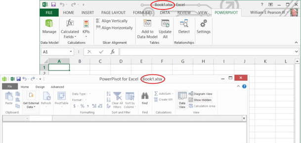
Illustration 3: The PowerPivot Window, Associated with the Workbook (Here, Book1.xlsx), Appears
As we noted in Level 1: Getting Started with PowerPivot and DAX, it is in the PowerPivot window that we load and prepare the data with which we will be working (or will continue working, if data is already added to the workbook). We will typically build a relational model here (even when we import other-than-relational sources, such as Analysis Services data, text files, .RSS feeds, and so forth). As we also noted in Level 1, the PowerPivot window displays the tables on individual, tabbed sheets. This is the central place where we import tables, create relationships, maintain column data types and formats, and view the data that underlies our data model, among other actions.
Next, we’ll designate a source from which to import data.
- On the Home tab of the PowerPivot Window, click the downward-pointing selector arrow on the right side of the From Database button, within the Get External Data group on the ribbon.
- Select From SQL Server on the cascading menu that appears next, as shown.
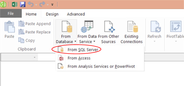
Illustration 4: Select “From SQL Server” in the Get External Data Dropdown Chain…
The Table Import Wizard dialog opens next.
- In the top input box, titled Friendly connection name, type (or copy and paste) the following (or another appropriate label):
AdventureWorksDW2012
- Click the selector (downward pointing arrow) on the right side of the box titled Server name.
PowerPivot begins a scan of the machine to detect, and return to the selector, the available server choices.
- Select the appropriate server for your local environment, or type in the server name / “localhost,” as appropriate.
- Enter the authentication as required for the local environment (ideally selecting Use Windows Authentication).
- Select AdventureWorksDW2012 (or your appropriately versioned equivalent) using the dropdown selector to the right of the box titled, Database name, at the bottom of the dialog.
The Table Import Wizard dialog, with our input, appears similar to that depicted below.
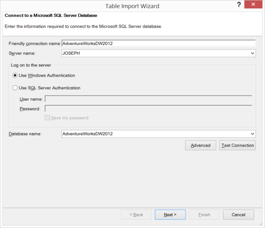
Illustration 5: The Table Import Wizard Dialog, with Our Input
- Click the Test Connection button underneath the Database name selector.
A message box appears, indicating that the test connection has succeeded.
Illustration 6: “Test Connection Succeeded”
- Click OK to dismiss the message box.
- Click the Next button at the bottom of the Table Import Wizard dialog.
- On the dialog that appears next, labeled Choose How to Import the Data, leave the radio button at its default of Select from a list of tables and views to choose the data to import, as shown.
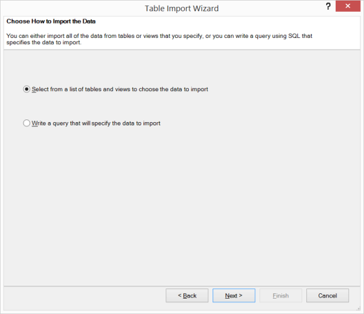
Illustration 7: Choose “Select from a list of tables…” Option for Data Import
- Click the Next button.
PowerPivot loads the tables and views from the AdventureWorksDW2012 database into the Select Tables and Views page that appears next.
- Select each of the tables listed in Table 1 by clicking the checkbox to the immediate left of the respective table listing in the Source Table column of the dialog, and change its name, via the Friendly Name in the dialog.
| Table to Select (Source Table) | Change Name to (Friendly Name): |
| DimCustomer | Customer |
| DimDate | Date |
| DimProduct | Product |
| DimProductCategory | Product Category |
| DimProductSubcategory | Product Subcategory |
| DimPromotion | Promotion |
| DimReseller | Reseller |
| FactInternetSales | Internet Sales |
| FactResellerSales | Reseller Sales |
Table 1: “Select Table and Views” Dialog Input
The Select Tables and Views dialog appears, as partially shown, with the tables listed selected and designated with their new names.
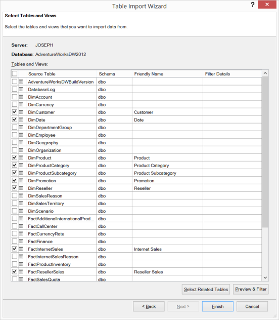
Illustration 8: Selecting Tables (Partial View)…
The idea in these immediate steps, once again, is to import enough information into our model to allow us to do some illustrative analysis surrounding the business activities conducted by our hypothetical client, the Adventure Works Cycles organization.
- Click the Finish button.
The import process runs, and then we see a “Success” message, complete with a Details list that indicates population by our choices.
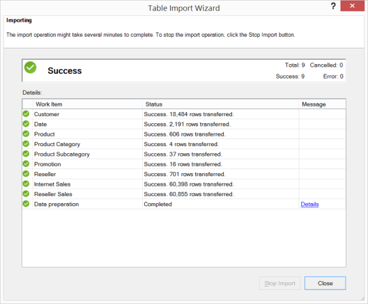
Illustration 9: Success is Indicated, Along with a List of Tables Imported
- Click Close.
The Table Import Wizard is dismissed, and we arrive at the PowerPivot window once again, where we see the imported data as partially depicted.
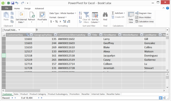
Illustration 10: Imported Data, with a Tab for Each Table (Partial View)
Note that a tab for each imported table has been created in the PowerPivot window (the tabs appear in the bottom left of the window, as seen above). What we are now seeing are not Excel tables / spreadsheets, but a view of the efficiently compressed columnar database that PowerPivot uses to store imported tables in memory. For more detailed information about the PowerPivot window itself, please see Level 1: Getting Started with PowerPivot and DAX.
- Click File, to the immediate left of the Home tab.
- Select Save As from the dropdown menu that appears, as shown.
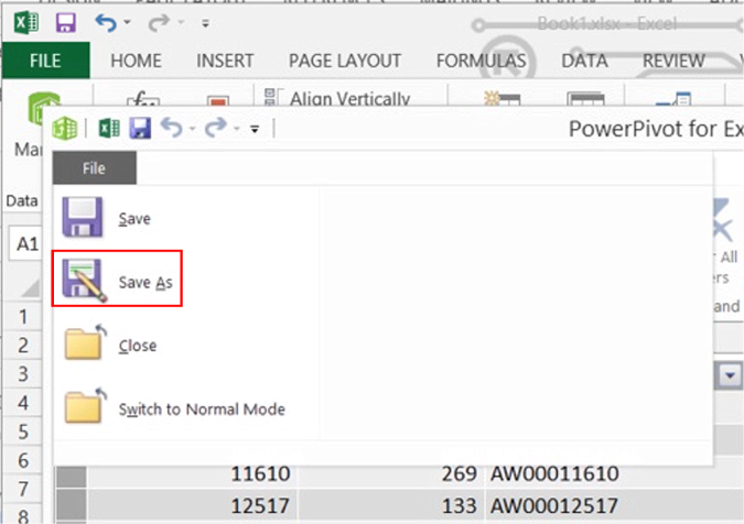
Illustration 11: Select Save As from the Selector within the PowerPivot Window…
- Save the worksheet as ST_DAX07-1.xlsx, placing it in a convenient location.
- Leave the PowerPivot Window open for the practice session below.
We are ready, at this stage, to get some hands-on exposure to another couple of DAX functions, AVERAGE() and AVERAGEX(). We will also revisit functions that we introduced in previous levels, while continuing to build experience with the general use of PowerPivot for Excel to meet business requirements, in the sections that follow.
The AVERAGE() Function
Introduction
According to the TechNet Library, the DAX AVERAGE() function “returns the average (arithmetic mean) of all the numbers in a column.” AVERAGE() is a member of the Statistical function group, as displayed in the formula bar for PowerPivot and PowerPivot PivotTables, many of the members of which are identical to functions in Excel. The function is often used in combination with other DAX functions.
Many of us have worked with the AVERAGE() function in standard Excel, where, like SUM(), it is a relative “cornerstone” function. And, while anytime we drag a field into a PivotTable (either a “classic” PivotTable or a PowerPivot PivotTable) Values drop zone, the default summary that is applied is Sum, we can choose from other treatments, including Average, as we can verify by right clicking upon the newly created sum of a value we have dropped into the Values drop zone, and then selecting Summarize By (whereby we can change the type of aggregation of a given Value). In the example below, we note the default behavior of the Sum option being checked as being in force, but that we can modify the aggregation behavior by selecting one of the other options appearing below Sum on the cascading menu.
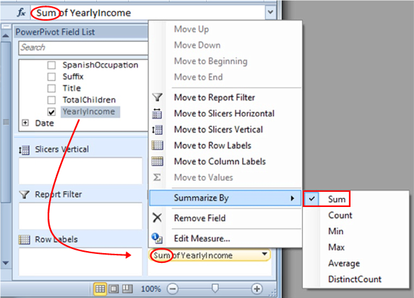
Illustration 12: Sum is the Default Treatment, but Average is among the Other Options…
AVERAGE() simply evaluates the numeric values residing in a column, and returns an average – a mean – of those values. In cases where there are no rows to average, AVERAGE() returns a blank. If rows do exist, but none of the rows meet the criteria for averaging, AVERAGE() returns a zero ( 0 ) value. With regard to nonnumeric values, the AVERAGE() function ignores any empty cells or logical values contained within the specified column.
When we employ AVERAGE() across date values, the returned result is a serial number. Moreover, no averaging action at all can be accomplished for a column that contains text, and, in such cases, AVERAGE() returns blanks. Finally, when cells containing a value zero (0) exist inside columns specified within the AVERAGE() function – as opposed to cells that are blank (which are not counted at all) – those cells are included: zeros are both added to the numerical total of the column and counted among the number of rows that comprise the divisor in the calculation of the mean.
It is significant to note that the AVERAGE() function calculates the average of all values (with the above noted exceptions) in a specified column – if a need exists to determine the average of an expression that evaluates to a specified set of numbers, we can do so via the AVERAGEX() function (discussed in its own section of this Level).
We will explore the syntax for the AVERAGE() function after a brief discussion in the next sections. We will then gain some hands-on exposure to its use, within practice examples constructed to support hypothetical business needs, in the Practice section later in this Level. This will allow us to activate what we explore in the Discussion and Syntax sections.
Discussion
To restate our initial explanation of its operation, the AVERAGE() function returns the mean of all the numeric values in the specified column. The output of AVERAGE() is a decimal number representing the arithmetic mean of the numbers in the column, and the function can be used with equal utility within PowerPivot calculated columns or PivotTable measures. AVERAGE() is often employed within other DAX functions.
NOTE: As we address in the section below, the AVERAGEX() function allows us to extend the operation of AVERAGE(), and take, as an argument, an expression that is, in turn, evaluated for each row in a table. This enables us to perform independent calculations, and to subsequently take an average of the calculated values that are returned, and to thus extend the logic of what we wish to average within a given set of values, by allowing us to specify an expression, which can represent an independent calculation, over which to apply the averaging action.
Syntax
Syntactically, in using the AVERAGE() function to return a mean, we specify the column of values we wish to average within the parentheses to the right of the AVERAGE keyword. As an illustration, we’ll cite the use of AVERAGE() within the Reseller Sales tab of the PowerPivot window which we have established in our earlier preparation. Let’s say we employ AVERAGE(), via a calculated column, in the following manner to average all numbers resident in the ProductStandardCost column:
=AVERAGE('Reseller Sales'[ProductStandardCost])
Were we to examine the new calculated column on the tab, we would see something like this (I’ve inserted the calculated column in the tab to be adjacent to the ProductStandardCost column, from which it is derived):
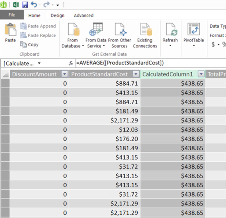
Illustration 13: Calculated Column Using AVERAGE() on the Reseller Sales Tab (Partial View)
Reaching beyond the partial view we see above, and extending to all rows in the column, the calculation returns the desired outcome, based upon the averaging of all the values contained in the ProductStandardCost column.
The AVERAGEX() Function
Introduction
According to the TechNet Library, the DAX AVERAGEX() function ”can take as its argument an expression that is evaluated for each row in a table. This enables you to perform calculations and then take the average of the calculated values.” Like AVERAGE(), AVERAGEX() is an “aggregate” member of the Statistics function group, as displayed in the formula bar for PowerPivot and PowerPivot PivotTables, many of whose members are identical to functions in Excel. AVERAGEX(), like other iterator (“X”) functions, and by its very nature, lends itself to use in combination with other DAX functions.
Iterator functions typically contain a table expression (the first parameter specified within the function), for which a calculation, based upon an expression specified by a second parameter, is performed iteratively for each row of the table. The ultimate result is generated by the application of the respective aggregation function (including SUM, AVERAGE, COUNT, MAX, and MIN) to the dataset returned by the first and second expressions. We expose the behavior of other DAX “X” functions in independent examinations of each of the respective function / x-function pairs published in parallel to this review of the AVERAGE() and AVERAGEX() functions.
In cases where there are no rows to average, AVERAGEX() returns a blank. If rows do exist, but none of the rows meet the criteria for averaging, AVERAGEX() returns a zero ( 0 ) value. With regard to nonnumeric values, the AVERAGEX() function ignores any empty cells or logical values contained within the specified column.
No averaging action at all can be accomplished for a column that contains text, and, in such cases, AVERAGEX(), like AVERAGE(), returns blanks. Finally, when cells containing a value zero (0) exist inside a column specified within the AVERAGEX() function – as opposed to cells that are blank (which are not counted at all) – those cells are included: they are both added to the numerical total of the column and counted among the number of rows that comprise the divisor in the calculation of the mean.
AVERAGEX() is useful anytime we want to filter a table we specify, based upon criteria we specify in a second expression, and then return an average of all the values in the resulting column. If we do not need to filter, we use the DAX AVERAGE() function, which, like SUM(), is similar to the Excel function of the same name, except that it references a column, versus a range.
We will briefly discuss the AVERAGEX() function in the section that follows, after which we will explore AVERAGEX() from a syntax perspective. We will then activate what we have explored in the Discussion and Syntax sections, through hands-on exposure to its use, within practice examples constructed to support hypothetical business needs.
Discussion
As we have noted, the AVERAGEX() function iterates through a specified table expression – taking it as its initial parameter, as it were. It then employs the second parameter, a column (or an expression that delivers scalar output) for which we seek to generate a mean, performing the expression for each row, and then averaging all the respective results obtained.
Let’s look at some syntax illustrations to further clarify the operation of AVEFRAGEX().
Syntax
Syntactically, in using the AVERAGEX() function to evaluate expressions for each row of a table, and then take the resulting set of values and calculate its arithmetic mean, we take a table expression (first argument of the function), and the expression (second parameter of the function) that we seek to apply to each row of the table (specified in the first argument), within parentheses, to the right of the AVERAGEX keyword. The general syntax is shown in the following string:
AVERAGEX(<table>, <expression>)
Putting AVERAGEX(), or any of the “X iterator” functions, for that matter, to work is intuitive, once we grasp the purpose. When using the function to return the average of the results of the action of the expression (“<expression>” in the syntax string above) upon each of the rows of the specified table (“<table>” in the syntax string above), we simply enclose the table and expression to the right of the AVERAGEX keyword, as we have noted. The AVERAGE function is then applied to the values returned for the respective rows, resulting in a single value that represents an average (mean) of those values.
As an example, let’s get a feel for the general use of AVERAGEX() within the Reseller Sales tab of the PowerPivot window, where we have performed the imports described in the Preparation section above. Let’s say we want to put AVERAGEX() to use in a scenario where we wish to do something along the lines of this:
=AVERAGEX('Reseller Sales', 'Reseller Sales'[SalesAmount] + 'Reseller Sales' [TaxAmt])
This calculates the average, combined Sales Amount and Tax Amount on each order in the Reseller Sales table, by initially summing Sales Amount and Tax Amount within each row, and then performing an average of all those sums. A partial view of the results of this calculation appears as shown:
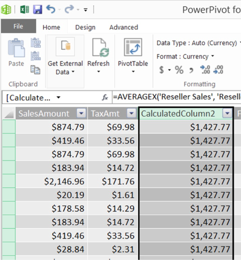
Illustration 14: AVERAGEX() Results: Average of the Sums of the SalesAmount and Tax Amount for Each Row for All Rows in the Reseller Sales Tab (Partial View)
In this simple example, we can see how AVERAGEX() allows us to extend the operation of AVERAGE(), and take, as an argument, an expression that is, in turn, evaluated for each row in a table (in this case, 'Reseller Sales'[SalesAmount] + 'Reseller Sales' [TaxAmt] ) . This capability enables us to perform independent calculations, and to subsequently take an average of the calculated values that are returned, as we have noted. We would control order of calculations by using parentheses, in cases where we use multiple operations in the expression used as the second argument.
We’ll get some hands-on practice with AVERAGE() and AVERAGEX() in the sections that follow.
Practice
Let’s reinforce our understanding of the basics by putting the AVERAGE() and AVERAGEX() functions to work within the definition of some calculations. We’ll do this much as we have in the other Levels of the Stairway to PowerPivot and DAX series, first via calculated columns within a tab of the PowerPivot window, and then via calculated fields within a PivotTable of a worksheet within the associated Excel workbook.
Also in keeping with our approach in other Levels of the series, we will examine the use of each of the functions in combination, where useful, with functions we have introduced in earlier Levels. The intent, as in all the practice sessions we undertake together within this series, is to demonstrate the operation of the functions we examine in a straightforward, memorable manner. We will turn to the Excel worksheet we prepared earlier as a platform from which to construct and execute the DAX we examine, and to view the results we obtain.
PowerPivot Calculated Columns
Let’s start with a straightforward example: Let’s say that we wish to perform a simple summarization to obtain the average Sales Amount on the Internet Sales tab within the PowerPivot data sheet view that we established in our preparation steps earlier.
To do so, we will take the following steps:
- Return to the worksheet we created in the Preparation for the Practice Exercises in this Level section above, ensuring that the PowerPivot Window is open, where we left it earlier.
- Click the Internet Sales tab.
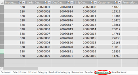
Illustration 15: Click the Internet Sales Tab…
- Click the heading of the column labeled “TaxAmt,” which appears to the immediate right of the SalesAmount column on the Internet Sales tab, as shown.
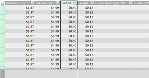
Illustration 16: Click the Heading of the Column Labeled “TaxAmt”
- Right-click the column label for the TaxAmt column.
- Select Insert Column from the context menu that appears.
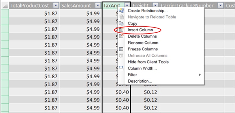
Illustration 17: Click Insert Column on the Context Menu…
A new calculated column, labelled CalculatedColumn1, appears.
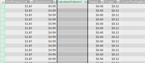
Illustration 18: A New Calculated Column Appears…
- Select the function button (“fx”) to the left of the formula bar next.
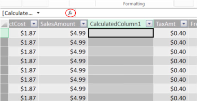
Illustration 19: Select the Function (fx) Button…
The Insert Function dialog appears.
- Click the downward pointing arrow on the selector appearing atop the dialog under the Select a category label.
The following DAX function categories appear:
- All
- Date & Time
- Math & Trig
- Statistical
- Text
- Logical
- Filter
- Information
- Parent-Child
- Select the Statistical category, on the Select a category dropdown, as depicted.
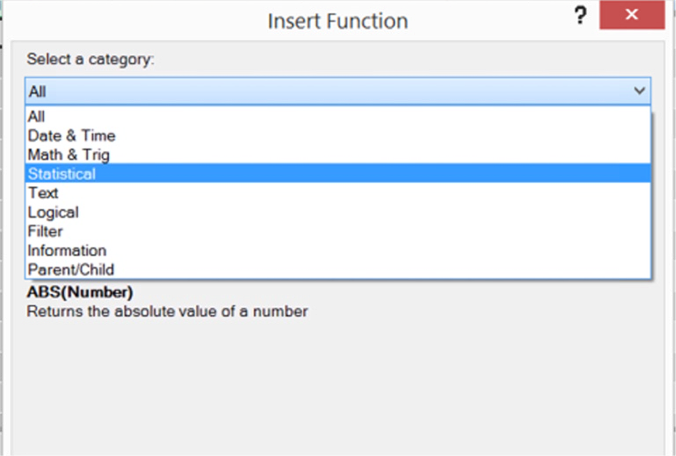
Illustration 20: Insert Function Dialog with Expanded Category Selector
- In the Select a function list that populates for the Statistical category, select the AVERAGE() function, as shown.
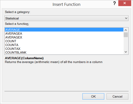
Illustration 21: Select the AVERAGE() Function
- Click OK to confirm the selection and dismiss the Insert Function dialog.
The AVERAGE keyword, proceeded by the “=” operator and followed by a left parenthesis ( “(“ ), appears in the formula bar, with a function usage tooltip appearing just underneath the function.
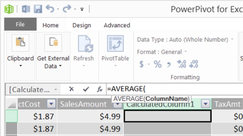
Illustration 22: The Beginning of A Calculation Using AVERAGE(), along with Tooltip, Appears
We will first create a simple calculation that generates an average / mean of the entire Sales Amount column of the Internet Sales tab, which we will name “Average Internet Sales.”
- Following the left parenthesis inserted by our selection of AVERAGE, begin to type in the word “InternetSales.”
- Scroll down and select ‘Internet Sales’[SalesAmount] within the dropdown list, then double-click / select the column.
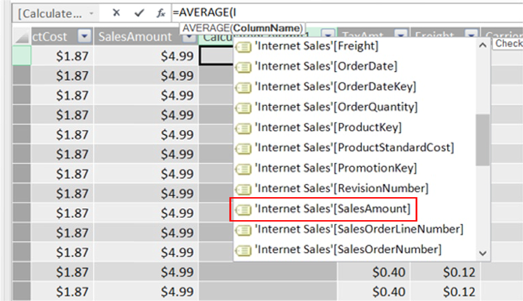
Illustration 23: Select the ‘Internet Sales’[SalesAmount] Column…
- Once the selector is dismissed, and =AVERAGE('Internet Sales'[SalesAmount] appears in the formula bar, type a right parenthesis ( “)” ) at the current end of the syntax, to close the AVERAGE() function.
The syntax, at this point, should be as shown here:
=AVERAGE(InternetSales[ExtendedSalesAmount])
- Once the syntax shown above appears in the formula bar, press the ENTER key.
The new calculated column is populated, in every row, by the averaging of all values in the Sales Amount column of the Internet Sales tab. Let’s name the column to something descriptive of its nature, at this juncture.
- Right-click the new column header label (currently at its default of “CalculatedColumn1”), and select Rename Column from the cascading menu that appears.
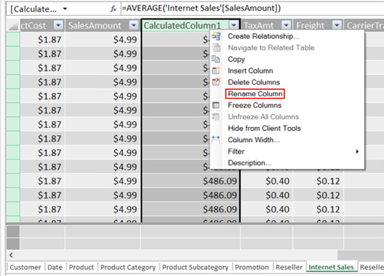
Illustration 24: Renaming the Column to its Intended Name
- Name the newly added column “Average Internet Sales” to provide a unique label.
The newly named column, with updated formula results, appears as partially depicted below.
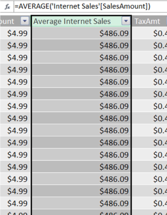
Illustration 25: The Results Appear in Each Row of the New Column (Partial View)
We thus see how we can employ AVERAGE() to deliver a simple arithmetic mean within the PowerPivot window. Next we’ll take a look at the same operation, in a similar scenario, using AVERAGEX().
AVERAGEX() the” X-function” version of AVERAGE(),is also a Statistical function. As we noted, in Level 6: Function / Iterator Function Pairs: The DAX SUM() and SUMX() Functions, was the case with the SUM() function, the AVERAGE() function, like other functions in both Excel and in DAX, is limited to the use of a single column as an argument. The X-function counterparts (this time, AVERAGEX() being the example) to several such “standard” functions (the respective example being AVERAGE(), in the present case) enable us to construct arguments with multiple columns.
Let’s look at a simple example that shows how we can use AVERAGEX() to aggregate the values generated by an expression returning an “Average Total Amount Billed,” consisting of an average of the addition of all the values in three columns. To do so, we’ll take the following steps from the Internet Sales tab:
- Click the top of the column labeled “CarrierTrackingNumber,” which appears three columns to the right of the Average Internet Sales column that we added, in earlier steps, to the Internet Sales tab, as shown.
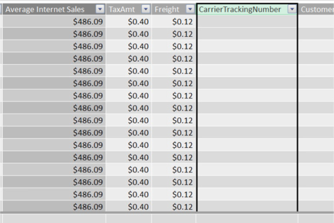
Illustration 26: Click the Top of the Column Labeled “CarrierTrackingNumber”
- Right-click the column label for the CarrierTrackingNumber column.
- Select Insert Column from the context menu that appears, as before.
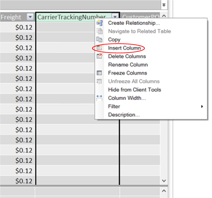
Illustration 27: Click Insert Column on the Context Menu, as Before…
A new calculated column, labelled CalculatedColumn1, appears, as we noted in earlier steps.
- Select the function button (“fx”) to the left of the formula bar next, as we did earlier.
The Insert Function dialog appears, once more.
- Click the downward pointing arrow, once again, on the selector appearing atop the dialog under the Select a category label.
- Select the Statistical category.
- In the Select a function list that populates for the Statistical category, select the AVERAGEX() function, as shown in Illustration 28.
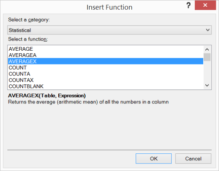
Illustration 28: Select the AVERAGEX() Function
- Click OK to confirm the selection and dismiss the Insert Function dialog, as we did earlier.
The AVERAGEX keyword, proceeded by the “=” operator and followed by a left parenthesis ( “(“ ), appears in the formula bar, with a function usage tooltip appearing just underneath the function, as we noted in working with the AVERAGE() function earlier.
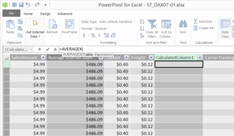
Illustration 29: The Beginning of Another Function, this time AVERAGEX(), along with Tooltip…
We will continue with the creation of another simple calculation (although, by the very nature of the AVERAGEX() function, slightly more sophisticated than the AVERAGE() function with which we worked earlier); this time, we will generate an “Average Gross Margin – All Products” that generates an average, across all products sold, of the “gross profit” (the Sales Amount minus the Total Product Cost) for each product transaction contained in the Internet Sales tab.
- Following the left parenthesis inserted by our selection of AVERAGEX, begin to type in the word “InternetSales,” once again.
- Scroll down and select the ‘Internet Sales’ table within the dropdown list to double-click / select the column, as depicted in Illustration 30.
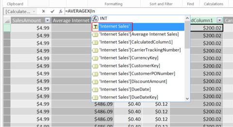
Illustration 30: Select the ‘Internet Sales’ Table, Once Again…
- Once the selector is dismissed, and =AVERAGEX('Internet Sales’ appears in the formula bar, type a comma ( “ , “ ) after 'Internet Sales’.
The syntax, at this point, should be as shown here:
=AVERAGEX('Internet Sales',
- After the comma that we have added at the end of the expression, type a left bracket ( “[“ ), and then begin to type in the word “SalesAmount”.
- Scroll down and select the [SalesAmount] column within the dropdown list to double-click / select the column, as shown in Illustration 31.
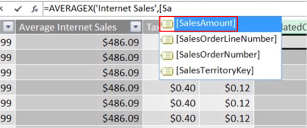
Illustration 31: Select the [SalesAmount] Column…
- Once the selector is dismissed, and =AVERAGEX('Internet Sales’,[SalesAmount] appears, type a minus sign ( “ - “ ) after [SalesAmount].
- After the “ - ” that we have added at the end of the expression, type another left bracket (“ [ “), and then begin to type in the word “TotalProductCost”.
- Select the [TotalProductCost] column within the dropdown list to double-click / select the column, as depicted.
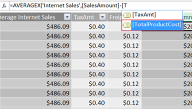
Illustration 32: Select the [TotalProductCost] Column…
- Once the selector is dismissed, and =AVERAGEX('Internet Sales’,[SalesAmount]-[TotalProductCost] appears, we have only to type a right parenthesis ( “ ) “ ) after [TotalProductCost] to close the AVERAGEX() function.
The syntax, in its final form, should be as shown here:
=AVERAGEX('Internet Sales',[SalesAmount]-[TotalProductCost])
The completed function appears as depicted in Illustration 33.
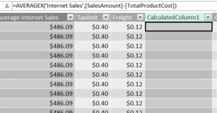
Illustration 33: The Completed AVERAGEX() Function
- Once the syntax shown above appears in the formula bar, press the ENTER key.
The new calculated column is populated, in every row, by the average of the “Sales Amount less Total Product Cost” calculations for all rows of the Internet Sales tab. Let’s name the column to distinguish it, once again, at this stage.
- Right-click the new column header label (currently at its default of “CalculatedColumn1”), and select Rename Column from the cascading menu that appears.
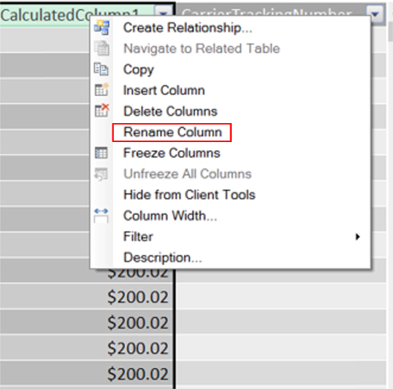
Illustration 34: Renaming the Column Label to Something More Meaningful…
- Name the newly added column “Average Gross Margin – All Products” to provide a unique column header name.
The newly named column, with updated formula results, appears as partially presented below.
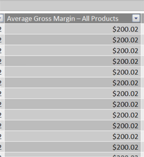
Illustration 35: The Results Appear in Each Row of the New Column (Partial View)
It’s easy to see how we can employ AVERAGEX(), in this simple scenario, to deliver an “average of calculation results” inside the specified Internet Sales table of the PowerPivot window.
Let’s look at one more example of the use of AVERAGEX(), via another calculated column in the Data Sheet View of PowerPivot. This time, we’ll exploit a slightly more sophisticated use of the second argument within the AVERAGEX() function. For purposes of this example, let’s say that we have been tasked with meeting a requirement to return an average value for a column within a given table, filtered for a given date only, via the DAX FILTER() function. To be specific, let’s say that the requirement is to return the average of the Sales Amounts of sales transacted on Order Date November 1, 2005, within the Reseller Sales table of the existing PowerPivot model. To achieve this, we will take the following steps:
- From within the Data Sheet View, click the Reseller Sales tab.
- Click the top of the column labeled “TaxAmt” (the column to the immediate right of the SalesAmount column) on the Reseller Sales tab, as shown.
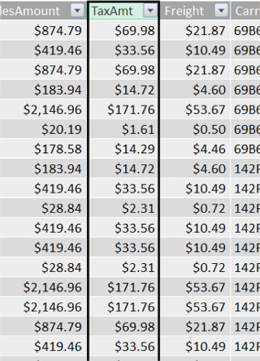
Illustration 36: Click the Top of the Column Labeled “TaxAmt”
- Right-click the column label for the TaxAmt column.
- Select Insert Column from the context menu that appears, as before.
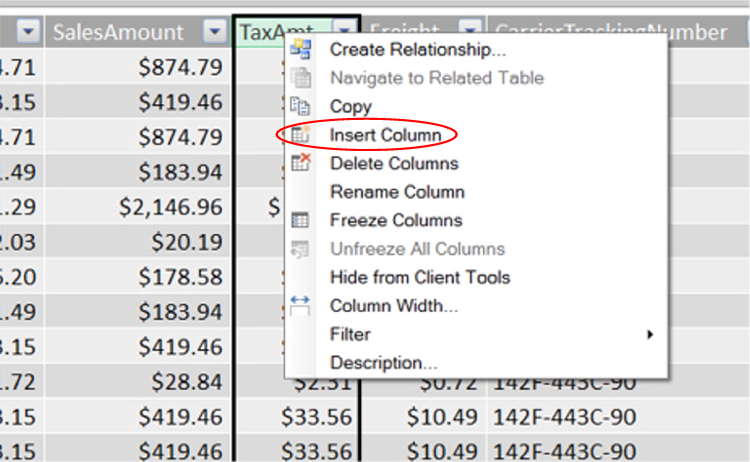
Illustration 37: Click Insert Column on the Context Menu, Once Again…
- A new calculated column, labelled CalculatedColumn1, appears, as we noted in earlier steps.
Select the function button (“fx”) to the left of the formula bar next, as we did earlier.
The Insert Function dialog appears, once more.
- Click the downward pointing arrow, once again, on the selector appearing atop the dialog under the Select a category label.
- Select the Statistical category.
- In the Select a function list that populates for the Statistical category, select the AVERAGEX() function, as we did in earlier examples.
- Click OK to confirm the selection and dismiss the Insert Function dialog, once again.
The AVERAGEX keyword, again proceeded by the “=” operator and followed by a left parenthesis ( “(“ ), appears in the formula bar for the newly inserted calculated column.
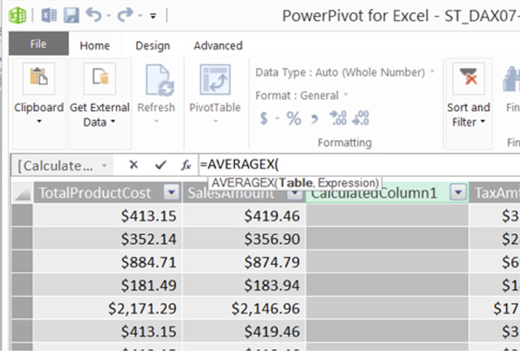
Illustration 38: The Beginning of an AVERAGEX() Function, along with Tooltip…
We will continue with the creation of another calculation – a calculation that performs the summation of the rows of a column, with the rows filtered for criteria that exists within another column, which we will specify in the second argument of the function.
- Following the left parenthesis inserted by our selection of SUMX, begin to type in the word “FILTER.”
- Select the FILTER function within the dropdown list by double-clicking the function, as depicted in Illustration 39.
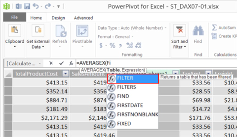
Illustration 39: Select the FILTER Function…
- Once the selector is dismissed, and =AVERAGEX(FILTER( appears, begin to type in the words “Reseller Sales.”
- Scroll down and select the ‘Reseller Sales’ table within the dropdown list to double-click / select the column, as shown.
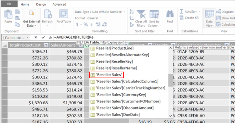
Illustration 40: Select the ‘Reseller Sales’ Table…
- Once the selector is dismissed, and =AVERAGEX(FILTER('Reseller Sales' appears in the formula bar, type a comma ( , ) after 'Reseller Sales’.
The syntax in the function bar, at this point, should be as shown here:
=AVERAGEX(FILTER('Reseller Sales',
- After the comma that we have added at the end of the expression, begin to type in the words “Reseller Sales,” once again.
- Scroll down and select the ‘Reseller Sales’[OrderDateKey] column within the dropdown list to double-click / select the column, as depicted.
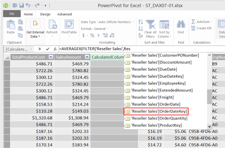
Illustration 41: Select the 'Reseller Sales'[OrderDateKey] Column…
- Once the selector is dismissed, and =AVERAGEX(FILTER('Reseller Sales', 'Reseller Sales'[OrderDateKey] appears, type an equals sign ( “=” ) after 'Reseller Sales'[OrderDateKey].
- After the “=” that we have added at the end of the expression, type the integer 20051101.
- Follow the integer 20051101 with a right parenthesis ( “)” ), and then a comma ( , ).
The syntax in the function bar, at this point, should be as shown here:
=AVERAGEX(FILTER('Reseller Sales', 'Reseller Sales'[OrderDateKey]=20051101),
NOTE: For a detailed explanation of the operation of the DAX FILTER() function, see Level 2: The DAX COUNTROWS() and FILTER() Functions and More About Calculated Columns and Measures.
- After the comma that we have added at the end of the expression, type in a left bracket ( “ [ “).
- After the left bracket just added, begin to type in the phrase “SalesAmount.”
- Select the [SalesAmount] column within the dropdown list by double-clicking, as shown.
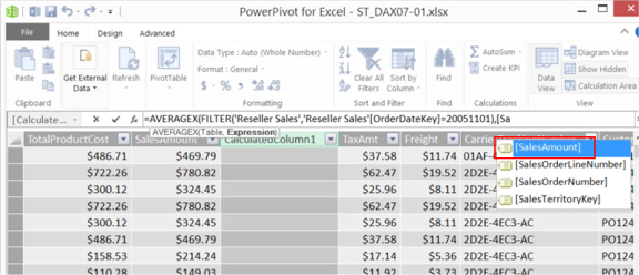
Illustration 42: [SalesAmount] Column…
- Once the selector is dismissed, and =AVERAGEX(FILTER('Reseller Sales', 'Reseller Sales'[OrderDateKey]=20051101),[SalesAmount] appears, type a right parenthesis ( “ ) “ ) after [SalesAmount].
The completed function should be as shown here:
=AVERAGEX(FILTER('Reseller Sales', 'Reseller Sales'[OrderDateKey]=20051101),[SalesAmount])
…and appears as presented in Illustration 43.
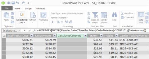
Illustration 43: The Completed AVERAGEX() Function
- Once the syntax shown above appears in the formula bar, press the ENTER key.
The expression we have assembled first filters the table, Reseller Sales, on the expression, OrderDateKey = 20051101, and then returns the average of all values in the column, SalesAmount. In other words, the expression returns the average of sales transactions for only the order date of November 1, 2005. Let’s name the column to distinguish it, as we have done with calculated columns we have created before.
- Right-click the new column header label (currently at its default of “CalculatedColumn1,” once again), and select Rename Column from the cascading menu that appears, as we have done in earlier examples.
- Name the newly added column “Average Sales Amounts 11-01-2005” to provide a unique column header name.
The newly-named column, with updated formula results, appears as partially shown.
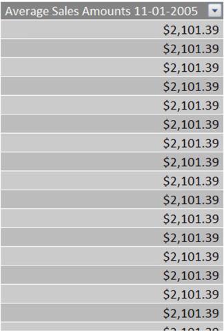
Illustration 44: The Results Again Appear in Each Row of the New Column (Partial View)
Let’s check our result with a simple test:
- On the Reseller Sales tab in the Data Sheet View, scroll over to the OrderDateKey column.
- Find a row in the OrderDateKey column where the value is 20051101, and then right-click on the cell containing that value.
- Select Filter --- > Filter by Selected Cell Value from the cascading context menus that appear, as shown.
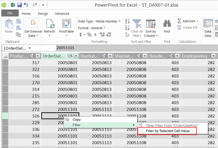
Illustration 45: Filter by Selected Cell Value…
The column is filtered to display only row items with 20051101 as the OrderDateKey.
- Scroll over to, and click on, the column label for the newly filtered SalesAmount column, selecting the column.
- Right-click the column heading.
- Select Copy from the context menu that appears, as depicted.
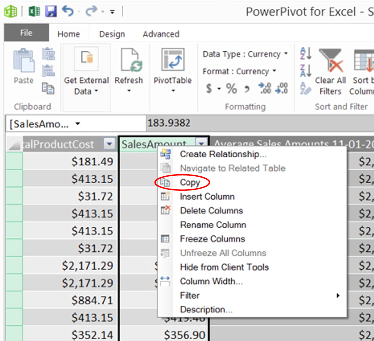
Illustration 46: Copy the Filtered SalesAmount Column…
- Click the Switch to Workbook button in the toolbar in the upper left corner of the PowerPivot Window, as shown, to return to the Excel workbook.
Illustration 47: Transit to the Excel Workbook
- Once the worksheet appears, right-click the cell in the upper left corner of the spreadsheet.
- Select the first of the two buttons appearing under Paste Options, on the context menu that appears next, as depicted.
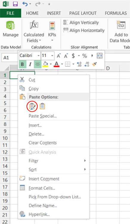
Illustration 48: Select the Left-most Paste Button to Paste…
The filtered SalesAmount column appears on the spreadsheet.
- Right-click the cell underneath the bottom cell of the new column, to select it.
- Click the downward pointing selector arrow on the right side of the Sum (Sigma, or “ S “) button on the Home toolbar.
- Select Average from the selector list to average the values above the chosen cell, as shown.
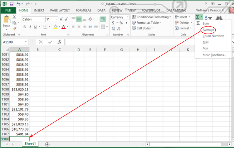
Illustration 49: Averaging the Filtered Column…
- Once the automatic average range appears in the cell, press the Enter key to generate the average of the values in the column.
We compare the average of the filtered SalesAmount column in the spreadsheet to the total generated by our most recent AVERAGEX() function in each row of the SalesAmount column on the Reseller Sales tab in the PowerPivot window, and see that the totals agree.
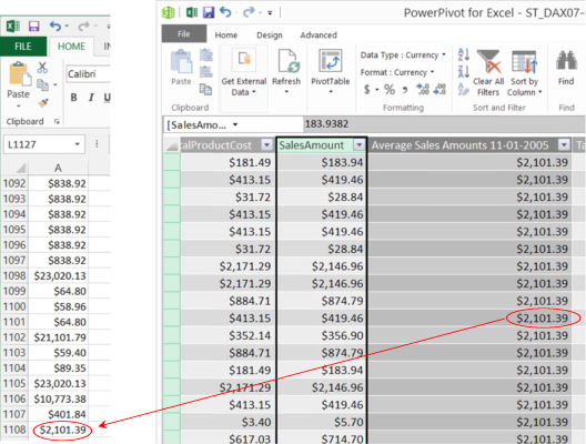
Illustration 50: Proving the AVERAGEX() Results in the Calculated Column in PowerPivot (Composite View)
So our “quick and dirty” test shows that the AVERAGEX() function has performed as expected.
- Clear the filter that we placed on the OrderDateKey column of the Reseller Sales table within the PowerPivot window.
In the section that follows, we will access the PowerPivot calculated columns we have created within a PivotTable. Moreover, we will get some hands-on exposure to putting the DAX AVERAGE() function to work within a calculated measure we will create in the PivotTable.
PivotTable Measure
We will next work further – this time via calculated fields (called measures in Excel 2010 PivotTables using PowerPivot data) - with the DAX functions we have exposed in the PowerPivot calculated column section above. We do this keeping in mind the assertion we make throughout the Stairway to PowerPivot and DAX series, that PowerPivot exists, in its fundamental role, to act as a data source for PivotTables,. The difference, this time, will be that we will present values and calculations within a PivotTable.
As most of us know by now, we can begin our work with a PivotTable from either the Excel workbook or from the PowerPivot window. Let’s return to the PowerPivot window (via the Manage button on the PowerPivot tab in Excel), and then proceed by taking the following steps:
- From the Reseller Sales tab in the PowerPivot window, click the downward pointing arrow on the PivotTable button to cause the drop-down menu to appear, as shown.
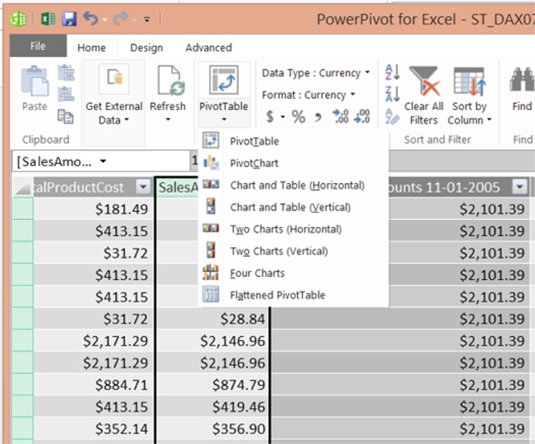
Illustration 51: The PowerPivot PivotTable Drop-down Menu Appears…
Although we work with examples, within various levels throughout our series, of some of the other options we see in the dropdown menu, we will build a couple of standalone PivotTables in this session. This will be the most efficient path to getting hands-on exposure to the underlying PowerPivot data and DAX, in general.
- Click PivotTable in the dropdown menu we’ve exposed (the top selection).
We are returned to Excel, where we encounter the Create PivotTable dialog.
- Ensure that the radio button labeled New Worksheet is selected, leaving the Location setting at default for now.
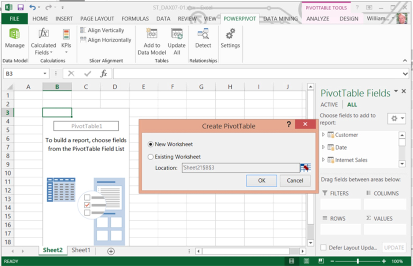
Illustration 52: Ensure the “New Worksheet” Option is Selected…
- Click OK to accept the setting and dismiss the dialog.
The PivotTable placeholder / canvas, together with the PivotTable Fields list, appear on the new worksheet as depicted (compressed view):
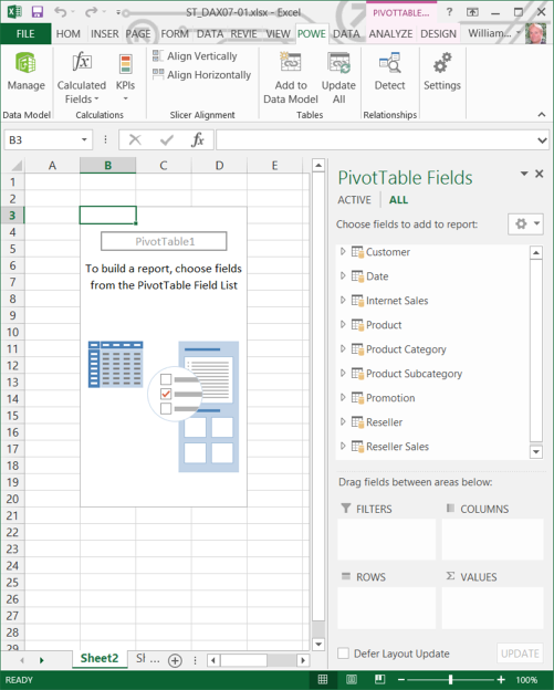
Illustration 53: The PivotTable Canvas Appears on the New Worksheet (Compressed View)
We’ll leave the placement of the new PivotTable at default.
NOTE: Because we cover the details for the first time in an earlier Level of the series, and particularly for those not already familiar with standard Excel PivotTables, Table 1 of Level 2: The DAX COUNTROWS() and FILTER() Functions and More About Calculated Columns and Measures gives a description for each of the areas / zones on the PivotTable Fields list. Other PivotTable basics are discussed there as well.
To gain some exposure to the use of the DAX AVERAGE() function within the PivotTable (our observations to the AVERAGE() function will apply to AVERAGEX(), as well), we will replicate some of the steps we took with regard to the Internet Sales and Reseller Sales tables, upon which we operated in the PowerPivot window in the earlier part of this Level. In accomplishing this, we’ll see how to approach what we did with the calculated column earlier, but this time we’ll do so with a calculated measure in the PivotTable. Moreover, we will touch upon more PivotTable – specific considerations as we encounter them. But first, we will pull calculations we created earlier into a new PivotTable we construct, to allow us to see the output of our calculation when we select it from the PivotTable Fields list.
- Expand both of the Product Category and Product Subcategory tables.
- Select the EnglishProductCategoryName and EnglishProductSubcategoryName from the Product Category and Product Subcategory tables, respectively, by placing a check in the associated checkboxes, as shown.
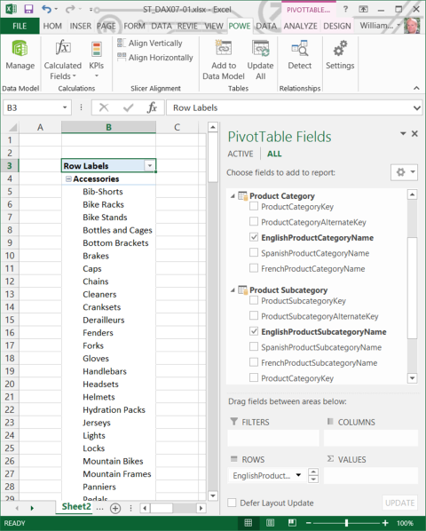
Illustration 54: Row Axis: Selections from the Product Category and Product Subcategory Tables
Our initial rows axis is in place at this stage. (This is, of course, behavior we have noted in articles throughout the series: the two selections we made were placed into the Row Labels drop zone of the PivotTable Fields list by default, as they are non-numeric values.) Now let’s add some values: calculated columns with which we worked in the PowerPivot window in our earlier sections.
- Expand the Internet Sales table in the Field List by clicking the “+” sign to its immediate left.
- Select the Average Internet Sales and Average Gross Margin – All Products from the Internet Sales table, in that order, by placing a check in the associated checkboxes, as shown.
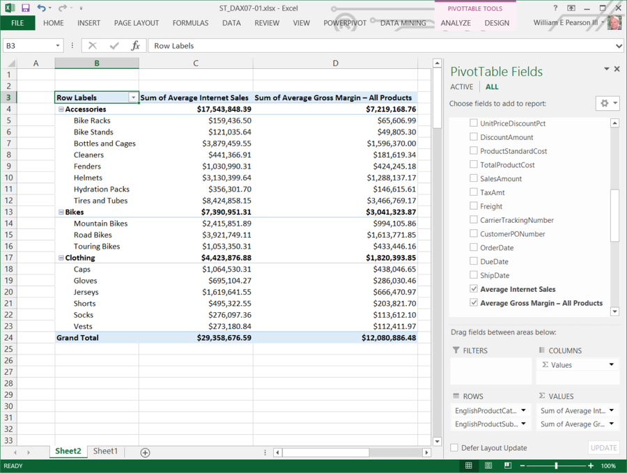
Illustration 55: Value Selections from Calculated Columns in the Internet Sales Table
Recall that the selections we have made from the Internet Sales table represent the calculated columns we created in the Internet Sales table of the PowerPivot Window. The first, Average Internet Sales, relies upon the DAX AVERAGE() function, the syntax of which is as follows:
AVERAGE('Internet Sales'[SalesAmount])
The second calculated column, Average Gross Margin – All Products, exploits the DAX AVERAGEX() function, using the following syntax:
=AVERAGEX('Internet Sales',[SalesAmount]-[TotalProductCost])
The PivotTable summary we have constructed to this point appears as shown:
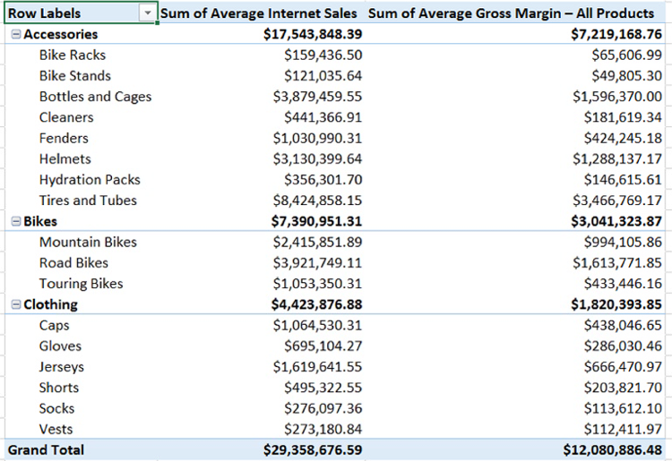
Illustration 56: PivotTable Summary with Calculated Columns Data from Internet Sales Table
We notice that the values presented in the columns, which we have populated by dragging the respective calculated columns into the PivotTable Values drop zone, seem quite large. To research why we have a difference, not to mention to ascertain which values are correct, let’s delve into the nature of our values a bit. The cause of the issue is largely indicated by the default names for the newly created values: Both have “Sum of” appended to the front of the names of the underlying calculated columns in PowerPivot. This is because values that are simply added to the Values drop zone (which is driven by the placement of the checkmarks to the left of the columns selected in the PivotTable Fields list) are summed, by default. Our indiscriminate dragging of the calculations to the Values drop zone has resulted in a default summation of an average – something that, on the surface, would be problematic.
Let’s see how changing this summing behavior to more accurately treat an average delivers immediate results – results that actually coincide with results that we can easily verify via the underlying PowerPivot calculation results. We’ll then take a look at recreating the Average Internet Sales calculation, currently a calculated column from the Internet Sales tab in the underlying PowerPivot Window that is pulled into the PivotTable, much as if it were any other column in the Internet Sales tab (there isn’t even any way to distinguish a calculated column from a standard column within the PivotTable Fields ist for the Pivot Table under examination).
Let’s make the tweak to more properly treat the Average Internet Sales calculation as an average, in general, as we have discussed.
- Within the Values drop zone of the PivotTable Fields list, click the downward pointing arrow on the value labelled Sum of Average Internet Sales.
- Select Value Field Settings from the menu that appears, as depicted here.
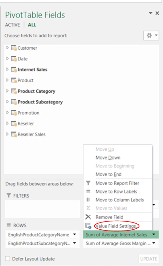
Illustration 57: Select Value Field Settings…
The Value Field Settings dialog appears, with settings as shown.
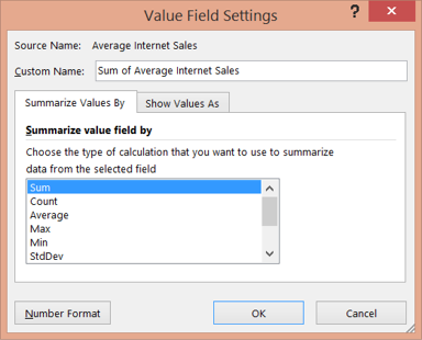
Illustration 58: Value Field Settings Dialog
Here we see that the Summarize value field by setting is Sum, as we discovered earlier.
- Modify the Summarize value field by setting to Average.
- Click OK to save changes and to dismiss the dialog.
We see immediate changes in the PivotTable:
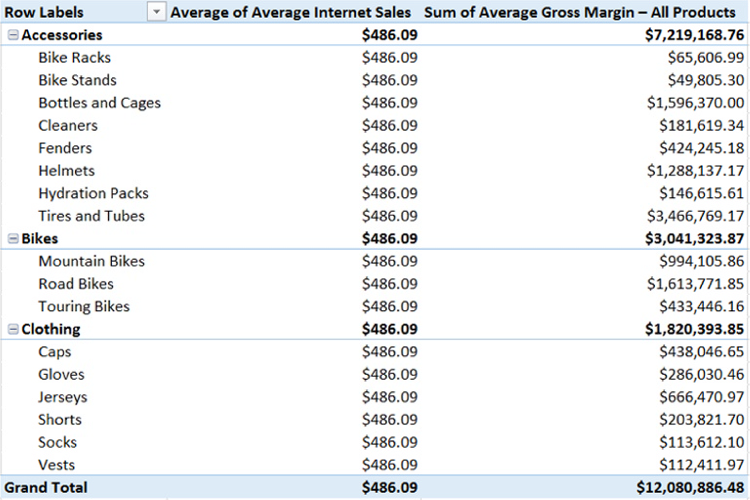
Illustration 59: PivotTable Summary with Modified Calculated Columns Data from Internet Sales Table
Depending upon the value we are attempting to generate in the PivotTable, this value is still not likely to be what we were expecting for every row – we would more likely have wanted to see an average column whose values are context sensitive to the respective Product Category / Product Subcategory row listings. For this, we will have to go beyond subjecting the PowerPivot AVERAGE() calculation to the average aggregation that we get by default here. We would have to do a little more work, via a calculated field that would generate the correct result.
Let’s add a calculated field in the PivotTable to give us a more meaningful average. We’ll leave the new Average of Average Internet Sales in place, for comparison purposes as needed.
- Click the PowerPivot tab, if necessary, atop the worksheet containing our current PivotTables.
- Click the Calculated Fields button in the ribbon atop the tab (to the right of the PowerPivot Manage button in the upper left of the ribbon).
- Select New Calculated Field… from the menu that appears, as presented here:
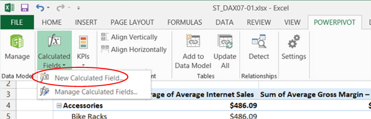
Illustration 60: Click New Calculated Field…
The Calculated Field dialog appears.
- Select Internet Sales in the dropdown selector labeled Table name atop the dialog.
- Type (or copy and paste) the following into both the Calculated Field Name box of the dialog.
Average Internet Sales CF
(We are simply naming the calculated field in a way to distinguish it from the entrained calculated column already in the PivotTable.)
- Click the function button (“fx”) to the right of the Formula label, above the Formula input box of the dialog.
The Insert Function dialog appears.
- Leave the Select a category label at the default setting of “All” this time.
- Scroll, within the Select a function dropdown, to the AVERAGE() function.
Select the AVERAGE() function, as depicted:
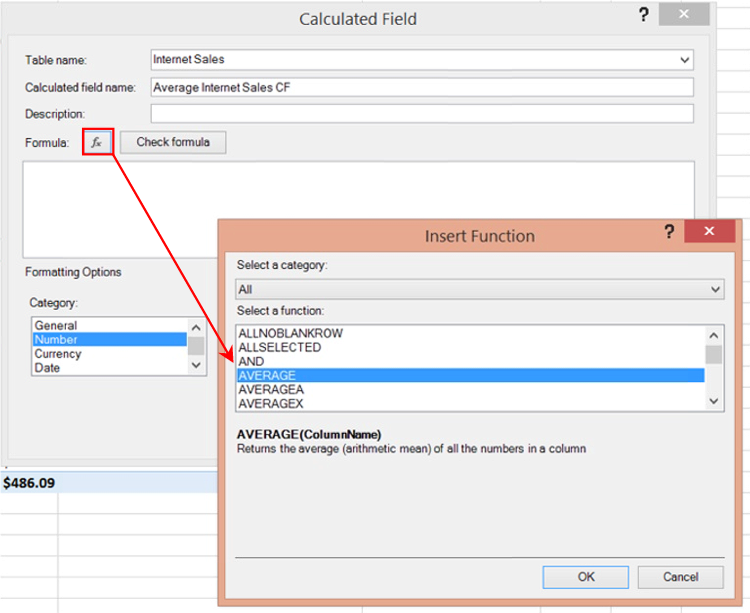
Illustration 61: Creating the New “Average Internet Sales CF” Measure…
- Click OK to confirm the selection and dismiss the Insert Function dialog.
The AVERAGE keyword, preceeded by the “=” operator, and followed by a left parenthesis, appears in the Formula input box of the Calculated Field dialog.
- To the immediate right of the left parenthesis (that appears to the right of the AVERAGE keyword), begin to type in “Internet Sales.”
As we begin to type the table name, AutoComplete again presents us with a list of selections that begin with Internet Sales, similar to the behavior to which we have become accustomed within the PowerPivot Window.
- Select ‘Internet Sales’[SalesAmount] from the dropdown selector, as shown.
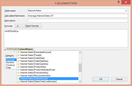
Illustration 62: Selecting the Desired Internet Sales Table Column…
The syntax in the function input box should appear, at this point, like this:
=AVERAGE('Internet Sales'[SalesAmount]
- Finally, add a right parenthesis ( “ ) “ ), to close the AVERAGE() function.
The syntax in the function input box should appear like this, at this point:
=AVERAGE('Internet Sales'[SalesAmount]
- Select Number in the Formatting Options section (the “Category” selections in bottom left corner) of the Calculated Field dialog, leaving the other formatting settings at default.
The Calculated Field dialog appears, with our input, as depicted.
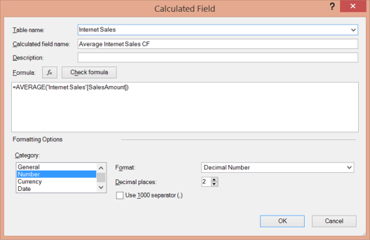
Illustration 63: The Calculated Fields Dialog, with Our Input
- Click OK to accept our input and dismiss the Calculated Field dialog.
The new calculated field, Average Internet Sales CF (which finds its home at the bottom of the member listings of the Internet Sales tree), appears within the Values drop zone automatically, as shown.
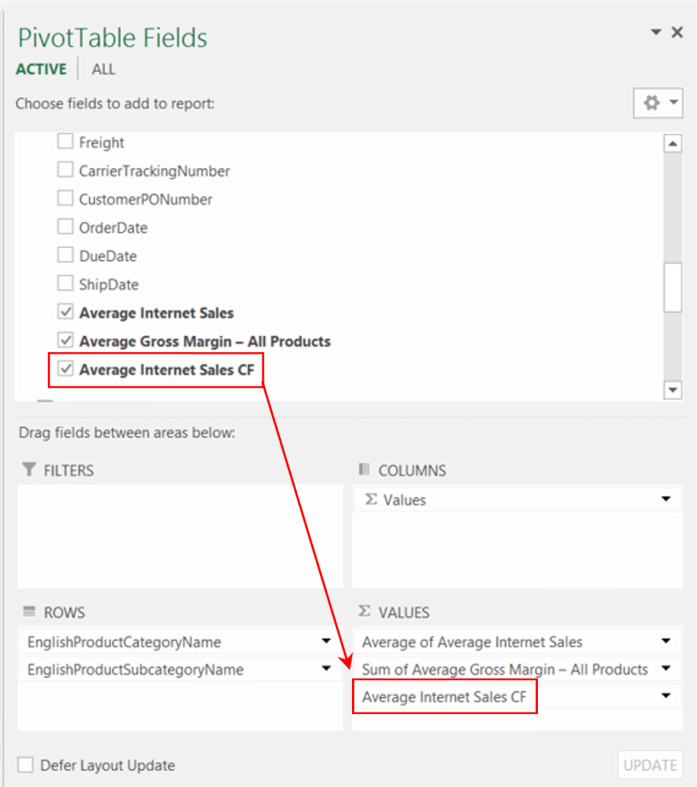
Illustration 64: The New Calculation Appears…
- Select and drag the Average Internet Sales CF calculation in the Values drop zone to be in between the two above it, Average of Average Internet Sales and Sum of Average Gross Margin – All Products.
At this juncture, the new Average Internet Sales CF calculation appears, within its home PivotTable, as shown:
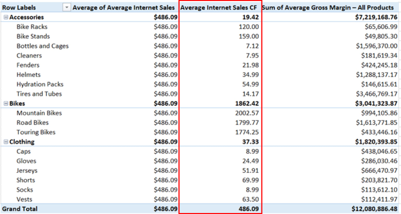
Illustration 65: The New Average Internet Sales CF Calculation Appears…
In this example, we once again illustrate the importance of “choosing the right calculation” (that is, choosing between a calculated column in PowerPivot and a calculated field in the PivotTable) for presentation in a PivotTable: While the new Average Internet Sales CF calculated field and the Average of Average Internet Sales value that appears to its immediate left share much the same logic, the huge difference in their presented values lies in the fact that the latter, a calculated column, is an “average of averages,” as we have discussed.
We can verify that the new Average Internet Sales CF calculation delivers results more along the lines of our probable desires with a simple, if somewhat manual, test. Let’s return to the PowerPivot window to proceed with the Mountain Bikes Product Subcategory as an example (the same logic will work for all Product Subcategories in the PivotTable we have constructed):
- Above the Excel ribbon on the spreadsheet where we now rest, from within the Home tab of a new worksheet, click the PowerPivot tab, as shown.
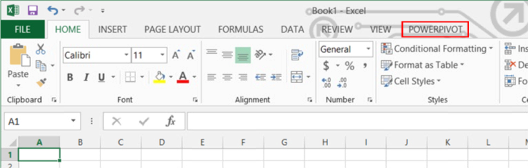
Illustration 66: Click the PowerPivot Tab within the Worksheet…
The PowerPivot ribbon appears.
- Click the Manage launch button, appearing at the left of the PowerPivot toolbar, as shown.
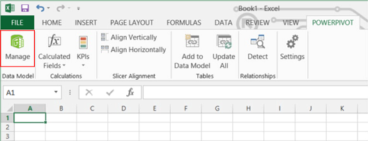
Illustration 67: The Manage Launch Button on the PowerPivot Ribbon…
Once we get to the PowerPivot Window, we’ll take teps to extract the set of sales transactions for the Mountain Bike Product Subcategory of the Bike Product Category.
- Click the Internet Sales tab to move to the Internet Sales data, once again.
- On the far left of the table, insert two calculated columns, Product Subcategory and Product Category, with the respective syntax as shown here:
- Calculated Measure Label: Product Subcategory
- Calculation Syntax:
=RELATED('Product Subcategory'[EnglishProductSubcategoryName])
- Calculated Measure Label: Product Category
- Calculation Syntax:
=RELATED('Product Category'[EnglishProductCategoryName])
Arrange the calculated columns in a manner similar to that shown in the partial view of the Internet Sales tab here:
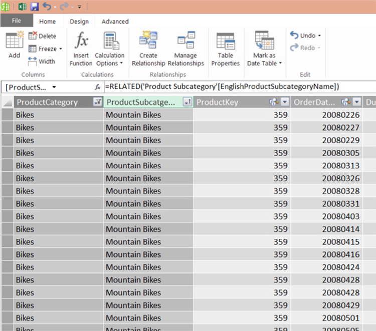
Illustration 68: Adding a Couple of “Helper” Calculated Columns…
NOTE: For a detailed overview of the DAX RELATED() function, see Stairway to PowerPivot and DAX - Level 1: Getting Started with PowerPivot and DAX.
- Click the sort / filter selector button on the right side of the new ProductSubcategory column label, as presented here:
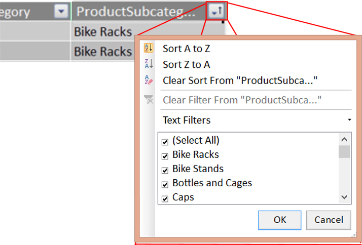
Illustration 69: Accessing the Sort / Filter Selector for the New ProductSubcategory Column…
- Uncheck (Select All) in the Text Filters box, and then check only the Mountain Bikes Product Subcategory, instead, as shown:
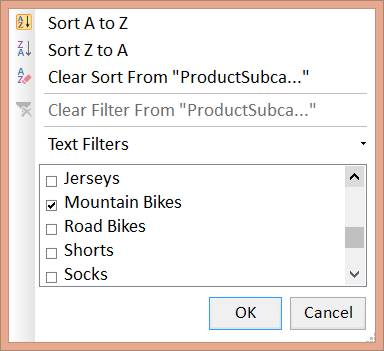
Illustration 70: Narrowing the ProductSubcategory Filter to Mountain Bikes…
This limits the Product Category selection to Bikes, as well.
- Click OK to accept changes, and to dismiss the selector.
The Internet Sales table flexes to fit our filter, leaving only the Bikes Product Category and the Mountain Bikes Product Subcategory among the rows displayed. We will now copy the Sales Amounts for these rows to a spreadsheet, where we can independently check that the Average Internet Sales CF calculation that we have created in the PivotTable is delivering accurate results.
- Click the (now-filtered) SalesAmount column on the Internet Sales table to select the entire column, as partially depicted in the illustration below.
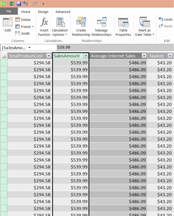
Illustration 71: Selecting the Entire SalesAmount Column of the Internet Sales Table….
- Leaving the SalesAmount column selected, click CTRL + C to copy the column.
- Click the Switch to Workbook button to return to Excel.
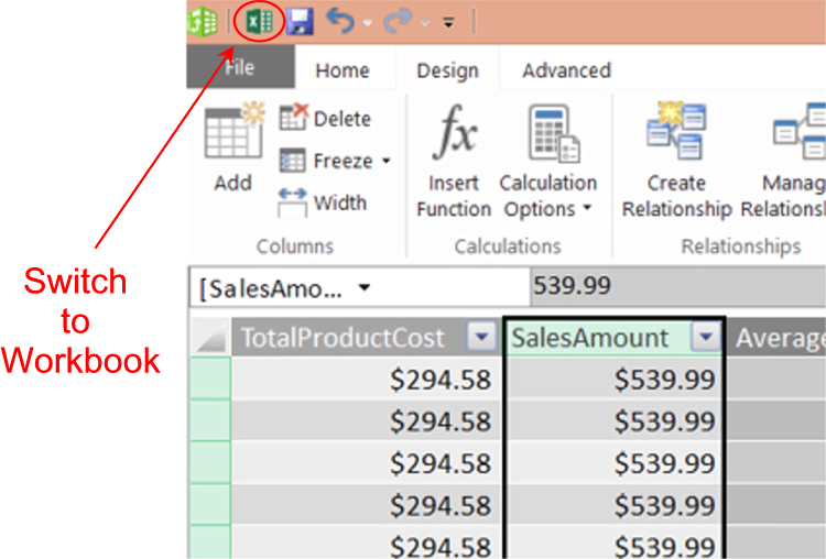
Illustration 72: Click the Switch to Workbook Button…
We arrive back in Excel.
- Create a new spreadsheet, if desired.
- Click a cell at the top of the spreadsheet, and then click CTRL + V to paste the copied column into the selected column of the spreadsheet.
- Once the values appear in the new column, scroll to the bottom of the data.
- In the cell beneath the last value, sum the values in the column, and then divide the total by 4970 (the number of values), using something like the following formula:
=SUM(A2:A4971)/4970
The value that is generated should approximate $2,002.57, as shown in the composite illustration below:
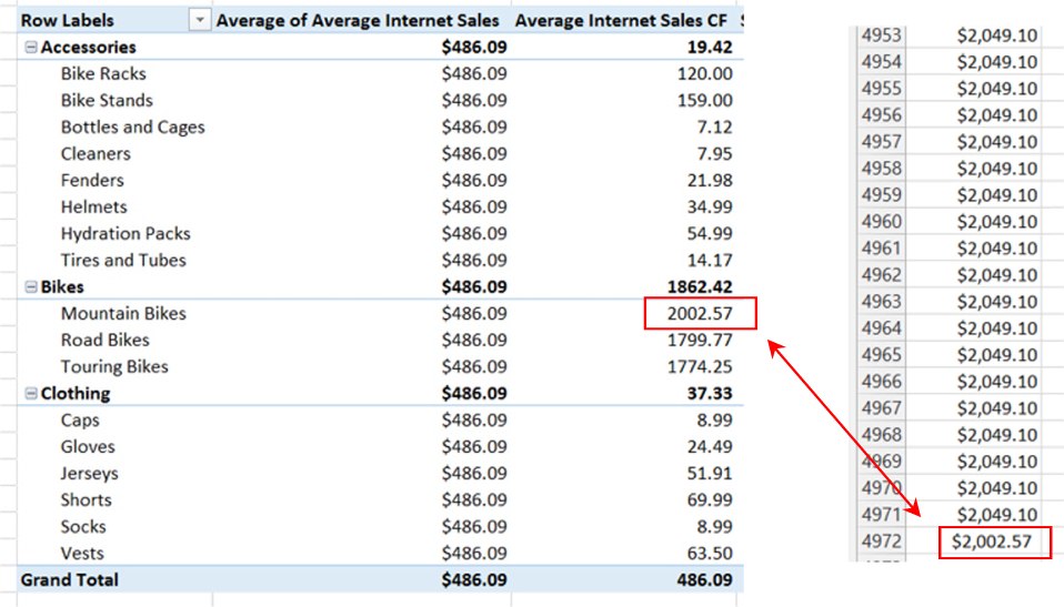
Illustration 73: Our Manual Calculation Supports the Results Produced by Average Internet Sale CF
We have noted in other Levels of this series that there are multiple things to consider in choosing “which total to use” (underlying, exposed calculated column or calculated field) in a given PivotTable, in similar cases. In this example, we can see that the “average of an average” is hardly likely to deliver the intended outcome.
The examples we have used with AVERAGE() and AVERAGEX() in this Step of the series are only relatively simple instances of what we can accomplish with their use. As we consistently note in other Steps, particularly where “X-” iterator DAX functions are involved, we can analyze and report upon data based upon date ranges, among other criteria, and create conditions (from simple to complex) that further refine the data, and / or include data taken from multiple tables. DAX empowers us to generate and support comprehensive BI within our Excel environments, transforming the relatively limited options we once had with simple spreadsheets into sophisticated and robust reporting and analysis solutions.
Summary
In this Level of the Stairway to PowerPivot and DAX series, we exposed the DAX AVERAGE() and AVERAGEX() functions. We discussed the general purposes and operation of each of these two DAX functions, and then focused upon using each in general, as well as comparing and contrasting ways that each can be employed, particularly in situations where we can combine them with other functions to achieve results like those we might need to generate in client or employer environments.
In like manner to our standard approach to every DAX function we explore within the Stairway to PowerPivot and DAX series, we examined the syntax surrounding each of the AVERAGE() and AVERAGEX() functions, undertaking illustrative examples of the uses of each in practice exercises, and then exploring the results datasets we obtained in the practice examples. We combined each of AVERAGE() and AVERAGEX() with other functions to deliver illustrative answers to business questions, within both PowerPivot calculated columns and PivotTable calculated measures we built in the section that followed. As we put calculations to use within the PivotTable, we compared and contrasted the values returned, explaining the reasons behind differences in the datasets they returned, and discussing considerations in choosing which calculation approaches to take in meeting business requirements in the business world.