
In this Level, we examine the DAX ISBLANK() function, which returns a “true” or a “false” from testing for a blank. As we learned in Level 4: The DAX BLANK() Function, and as we shall further discuss in the sections that follow, it is important to understand the nature and behavior of missing or empty values in a DAX expression before we can fully control its output. BLANK(), which we covered in Level 4 and will revisit here, and ISBLANK() are two important means of enforcing such control.
As a part of our exploration, we will discuss ways in which ISBLANK() can be employed, in situations where we combine it with other functions, to achieve a result similar to something we might need to generate for clients or employers in our own environments. During our exploration of the ISBLANK() function, we will:
- Discuss the nature of missing or empty values in a DAX expression;
- Examine the syntax involved in exploiting the function;
- Undertake illustrative examples of the uses of the function in practice exercises;
- Briefly discuss the results datasets we obtain in each of the practice examples.
As is standard procedure in my introductions to DAX functions within this Stairway series, we will examine the output we obtain, employing ISBLANK () via a calculated column we construct within the PowerPivot window in the practice session that follows. We will further create a measure that puts ISBLANK() to work in a PivotTable measure, to further scrutinize the behavior that we have examined in the calculated column created in the PowerPivot window. Moreover, as we have also consistently done within the Levels of this series, we will compare and contrast differences in use and behavior of the functions in calculated columns and calculated members in general, suggesting criteria to consider in choosing which of these calculation types to employ to meet the business requirements we encounter.
Preparation for the Levels of the Stairway to PowerPivot and DAX Series
To obtain the most benefit from the Levels of the Stairway to PowerPivot and DAX series, you will need to have installed the appropriate PowerPivot for Excel 2010 add-on on your machine. (You can also use Microsoft Office Excel 2013 to complete most steps of the levels of this Stairway, although naming conventions and screen appearances might differ a little from what you see in the articles of this series). In many cases, you will also need to have installed SQL Server 2008 or above (including Analysis Services) and the respective relational and Analysis Services samples on your local machine, or have the client portions of each on your machine, with access to the rest on a server. To perform all steps of preparation for the Levels of Stairway to PowerPivot and DAX, see the installation section of the charter Level of this series, Level 1: Getting Started with PowerPivot and DAX.
Preparation for the Practice Exercises in this Level
Once we’ve gotten the PowerPivot for Excel 2010 add-in (or have installed and configured Excel 2013), SQL Server 2008 (or above) and the samples noted above installed, we’re ready to perform the practice exercises within this Level. Importing the sample database and taking other preparatory steps are critical to providing the environment required to successfully complete this Level, and should be performed before beginning.
Because we will work with different data sources throughout this series, the steps of environment preparation will be repeated in various Levels – primarily to make each Level a freestanding session that can be completed independently of other Levels, so that you can focus upon gaining exposure to the specific skills required to meet your own immediate requirements efficiently. Where appropriate, references to functions, procedures and other details will be supplied, but the objective of each Level is to focus upon one or more specific DAX functions and / or PowerPivot / PivotTable procedures to satisfy needs that mirror requirements you encounter in our own business environments.
Let’s open PowerPivot and import our data by taking the steps below. This will put us in position to begin learning the material in this Level.
- From the Start menu, select Microsoft Excel.
- Above the Excel ribbon, within the Home tab of a new worksheet, click the PowerPivot tab, as shown.
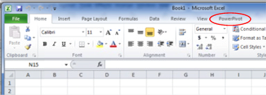
Illustration 1: Click the PowerPivot Tab within a New Worksheet
The PowerPivot ribbon appears.
- Click the PowerPivot Window launch button, appearing at the left of the newly appearing PowerPivot toolbar, as shown.
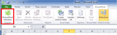
Illustration 2: The PowerPivot Window Launch Button on the PowerPivot Ribbon …
The PowerPivot window, containing its own ribbon, opens atop the existing Excel spreadsheet, assuming the name of the workbook as its own name, as depicted below.
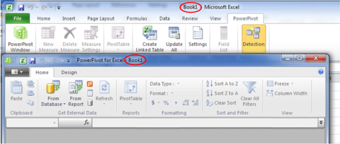
Illustration 3: The PowerPivot Window, Associated with the Workbook, Appears
As we noted in Level 1: Getting Started with PowerPivot and DAX, it is in the PowerPivot window that we load and prepare the data with which we will be working (or will continue working, if data is already added to the workbook). We will typically build a relational model here (even when we import other-than-relational sources, such as Analysis Services data, text files, .RSS feeds, and so forth). As we also noted in Level 1, the PowerPivot window displays the tables on individual, tabbed sheets. This is the central place where we import tables, create relationships, maintain column data types and formats, and view the data that underlies our data model, among other actions.
Next, we’ll designate a source from which to import data.
- Click the From Database button on the Home tab of the PowerPivot window.
- Select From SQL Server on the drop-down menu that appears next.
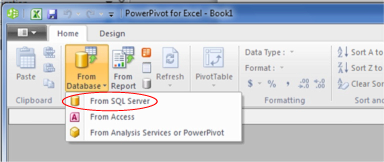
Illustration 4: Select “From SQL Server” in the From Database Dropdown
The Table Import Wizard dialog opens next.
- In the top input box, titled Friendly connection name, type (or copy and paste) the following:
AdventureWorksDW2008R2 - Click the selector (downward pointing arrow) on the right side of the box titled Server name.
PowerPivot begins a scan of the machine to detect, and return to the selector, the available server choices.
- Select the appropriate server for your local environment, or type in the server name / “localhost,” as appropriate.
- Enter the authentication as required for the local environment (ideally selecting Use Windows Authentication).
- Select AdventureWorksDW2008R2 using the dropdown selector to the right of the box titled, Database name, at the bottom of the dialog.
The Table Import Wizard dialog, with our input, appears similar to that depicted below.
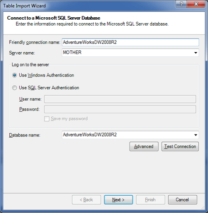
Illustration 5: The Table Import Wizard Dialog, with Our Input
- Click the Test Connection button underneath the Database name selector.
A message box appears, indicating that the test connection has succeeded.
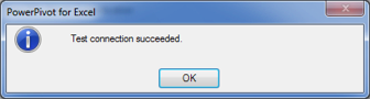
Illustration 6: “Test Connection Succeeded”
- Click OK to dismiss the message box.
- Click the Next button at the bottom of the Table Import Wizard dialog.
- On the dialog that appears next, labeled Choose How to Import the Data, leave the radio button at its default of Select from a list of tables and views to choose the data to import, as shown.
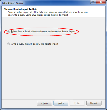
Illustration 7: Choose “Select from a list of tables…” Option for Data Import
- Click the Next button.
PowerPivot loads the tables and views from the AdventureWorksDW2008R2 database into the Select Tables and Views page of that appears next.
- Select each of the tables listed in Table 1 by clicking the checkbox to the immediate left of the respective table listing in the Source Table column of the dialog, and changing its name, via the Friendly Name in the dialog.
| Table to Select (Source Table) | Change Name to (Friendly Name): |
| DimCustomer | Customer |
| DimDate | Date |
| DimProduct | Product |
| DimProductCategory | Product Category |
| DimProductSubcategory | Product Subcategory |
| DimPromotion | Promotion |
| FactInternetSales | Internet Sales |
| FactResellerSales | Reseller Sales |
Table 1: “Select Table and Views” Dialog Input
The Select Tables and Views dialog appears, as partially shown, with the tables listed selected and designated for their new names.
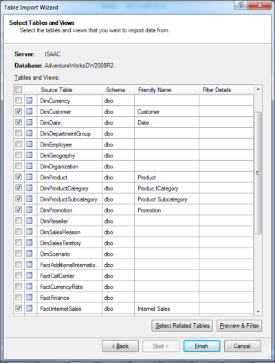
Illustration 8: Selecting Tables (Partial View)
The idea in these immediate steps, once again, is to import enough information into our model to allow us to do some illustrative analysis surrounding the business activities conducted by our hypothetical client, the Adventure Works Cycles organization.
- Click the Finish button.
The import process runs, and then we see a “Success” message, complete with a Details list that indicates population by our choices.
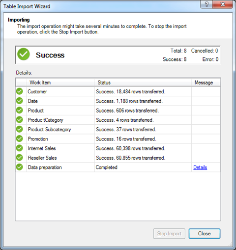
Illustration 9: Success is Indicated, Along with a List of Tables Imported
- Click Close.
The Table Import Wizard is dismissed, and we arrive at the PowerPivot window once again, where we see the imported data as partially depicted.
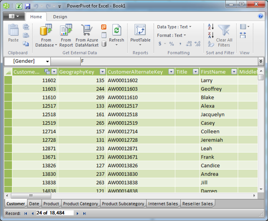
Illustration 10: Imported Data, with a Tab for Each Table
Note that a tab for each imported table has been created in the PowerPivot window (the tabs appear in the bottom left of the window, as seen above). What we are now seeing are not Excel tables / spreadsheets, but a view of the efficiently compressed columnar database that PowerPivot uses to store imported tables in memory. For more detailed information about the PowerPivot window itself, please see Level 1: Getting Started with PowerPivot and DAX.
- Click the selector underneath the Quick Access Toolbar (assuming it is in the default, above-the-ribbon position), and to the immediate left of the Home tab in the ribbon.
- Select Save As from the dropdown menu that appears, as shown in Illustration 11.
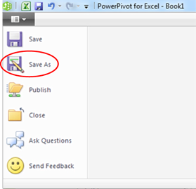
Illustration 11: Select Save As from the Selector within the PowerPivot Window
- Save the worksheet as ST_DAX05-1.xlsx, placing it in a convenient location.
- Leave the PowerPivot Window open for the practice session below.
We are ready, at this stage, to get some hands-on exposure to a new DAX function, ISBLANK(), which is related to the BLANK() function that we explored in Level 4: The DAX BLANK() Function. ISBLANK(), while revisiting functions that we introduced in previous levels, as well as continuing to build experience with the general use of PowerPivot to meet business requirements, in the sections that follow.
Before we dive into a hands-on exploration of these functions, though, let’s review what we learned in the earlier Level about how PowerPivot and Excel handle empty or missing values.
Empty Values
As a prelude to our examination of the nature and operation of the DAX ISBLANK() function, we’ll repeat a portion of our discussion, from Level 4: The DAX BLANK() Function, on how empty values are treated in PowerPivot and Excel. As we noted there, this becomes important because empty values often result in calculation errors and / or unexpected results. A good understanding of how empty or missing values behave in a DAX expression, as well as how we can use the BLANK() function to return an empty cell in a calculated column or in a measure, enables us to effectively control the results of a DAX expression under these conditions.
In SQL Server, as well as within most relational databases, a missing value is treated as “Null.” It is typical in relational environments for calculations involving a Null to return a Null by default, although SQL Server and other relational environment allow for modification of this behavior. In Analysis Services, as well as in other multidimensional databases, missing values are typically treated, depending upon the source data type, as empty strings or zeros.
PowerPivot designates a missing value as a “Blank.” When we add a number to a blank value, the number itself is returned, instead of a Null or another Blank. In handling missing values, blank values, or even empty cells, DAX uses a value of BLANK. BLANK comprises a way to identify these conditions, and is not a real value itself. To obtain a value of BLANK, which is different from an empty string, we employ the BLANK() function, as we described in Level 4: The DAX BLANK() Function. We often use BLANK() in conjunction with the ISBLANK() function for reasons that become apparent early.
Excel differs from PowerPivot in its treatment of empty values. Excel interprets an empty value as a zero (“0”) when that value is used within a summing or multiplication operation. Moreover, Excel returns an error if empty values are subjected to division, or used within a logical expression.
The ISBLANK() Function
Introduction
According to the TechNet Library, the DAX ISBLANK() function returns “a Boolean value of TRUE if the value is blank; otherwise FALSE.” ISBLANK() is a member of the information functions group, whose complex and powerful members enable us to manipulate data context to craft dynamic calculations. These functions are typically used in combination with other DAX functions; for example, ISBLANK() is very commonly employed as the first argument in the IF() function.
As we can see, ISBLANK() is useful to us in testing against empty values (called “Blank”) in DAX. When we supply an argument of Blank, as we shall see, ISBLANK() returns True when it detects a case of an empty value. The behavior of ISBLANK() becomes particularly important in scenarios where we encounter data where the meaning of a missing value is different from a zero (“0”) value.
We will explore the syntax for the ISBLANK() function after a brief discussion in the next section. We will then gain some hands-on exposure to its use, within practice examples constructed to support hypothetical business needs. This will allow us to activate what we explore in the Discussion and Syntax sections.
Discussion
To restate our initial explanation of its operation, the ISBLANK() function returns True or False, depending upon whether or not a value that it is being used to evaluate is blank. ISBLANK() is an Excel function that supports DAX.
Let’s look at some syntax illustrations to further clarify the operation of ISBLANK().
Syntax
Syntactically, in using the ISBLANK() function to return a True or False, with regard to the “blankness” of a given value, we specify the value we wish to test within the parentheses to the right of the ISBLANK keyword. As an illustration, let’s envision the use of ISBLANK() within the Customer tab of the PowerPivot window. Let’s say we wish to employ ISBLANK() to return, via a calculated column, the string “NMN” (an acronym for “No Middle Initial”), when the MiddleName column is blank, or the value within the MiddleName column when the column is populated.
=IF(ISBLANK(Customer[MiddleName]), "NMI", Customer[MiddleName])
If we looked at the new calculated column on the tab, at a point where we have incidents of the MiddleName column containing both single middle initials and Blanks, we would see something like this (I’ve moved the calculated column in the tab to be adjacent to the MiddleName column for easier visual verification):
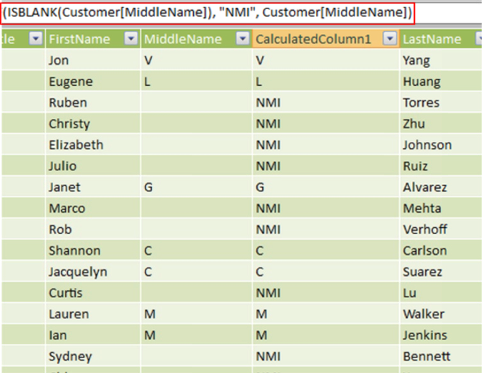
Illustration 12: Calculated Column Using ISBLANK() on the Customer Tab (Partial View)
As is obvious, within the compact view we see above, the calculation returns the desired outcome, based upon the True / False condition of “blankness.” The MiddleName column contains many Nulls. Because AdventureWorksDW2008R2 (the source of our import) is a SQL Server relational database, the Nulls are converted to Blank values. We are testing for Blank values with the ISBLANK() function, and employing IF() to evaluate whether the ISBLANK() function is returning True or False. If True is returned, the string “NMI” is returned. If a False is returned, the output is the content of the MiddleName column for the respective row.
Let’s get some hands-on practice with ISBLANK() in the section that follows.
Practice
As we do with all the DAX functions we introduce within the Stairway to PowerPivot and DAX series, we will reinforce our understanding of the basics by putting the ISBLANK() function to work within the definition of a couple of calculations, first via a calculated column within a tab of the PowerPivot window, and then via a calculated measure within a PivotTable of a worksheet within the associated Excel workbook. We will examine its use in combination, where useful, with functions we introduced in earlier levels of this series. The intent, as in all the practice sessions we undertake together within the series, is to demonstrate the operation of each of the functions we examine in a straightforward, memorable manner.
We will turn to the Excel worksheet we prepared earlier as a platform from which to construct and execute the DAX we examine, and to view the results we obtain.
PowerPivot Calculated Column
Let’s begin with a relatively simple example, wherein we deal with a scenario involving the “empty” values we touched upon earlier. Recall that database practitioners and the like call an empty value a “Null.” In their meaning, the column occupied by the Null contains no value – a value for this column being presumably optional, and a Null being the default “empty” value, as Nulls don’t unnecessarily consume space.
One of the inconveniences of having Nulls in place, however, is that the empty value it presents can lead to confusion for laymen report audiences: if we aggregate and present data based upon the members of the column, the Null values present a blank space to those viewing the summary. For purposes of our first practice example, let’s take a look at a straightforward way to make the presentation a little more user- friendly – via the ISBLANK() function.
Let’s say that we have been informed of a “Null scenario” by a client representative that matches the circumstances I’ve detailed above. While it is a reasonably appropriate scenario, it will help us to illustrate the presentation challenges. In the Product tab of the PowerPivot Window, we can see that the ProductLine column contains many empty rows – this makes sense, of course, as Bikes are the only kinds of products that correspond to a Product Line, as defined by Adventure Works Cycles. But, again, for purposes of this practice example, let’s manage those Nulls in a way that illustrates the use of ISBLANK().
Let’s say that the basic need is illustrated in the following simple PivotTable that the client representatives show us: From the PowerPivot Field List, Product table, they have selected ProductLine on the rows, and StandardCost into the values section, as shown.
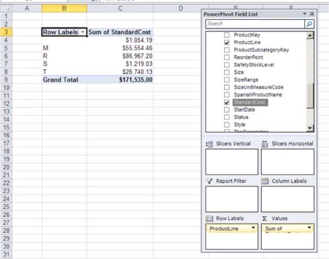
Illustration 13: Basic PivotTable, Illustrating “Blank” Summary Row
As we can see, the top row in the PivotTable is blank – due to the fact that many rows of the ProductLine column in the Product table, within the underlying PowerPivot window, are blank. While the lack of definition of ProductLine for many products likely makes sense within the Adventure Works inventory, we are merely using this scenario to illustrate a way around something that the information consumers find confusing: the lack of a label when no ProductLine is defined.
Our client colleagues tell us they would rather see the empty label contain “Unassigned,” so that report readers / analysts would know immediately that that respective row presented a summary for products without product line assignments. Because we know that the “blank” row exists because of “empties” in the underlying ProductLine column, we can handle the support of an “Unassigned” label via the ISBLANK() function.
Under these circumstances, a straightforward approach to meeting the business need is to create a calculated column, in the PowerPivot data sheet view, to “reclassify” the blank rows in the ProductLine column as “NA,” while leaving all rows containing a ProductLine “as is.” To do so, we take the following steps:
- Return to the worksheet we created in the Preparation for the Practice Exercises in this Level section above, ensuring that the PowerPivot Window is open, where we left it earlier.
- Click the Product tab.
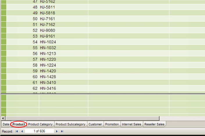
Illustration 14: Click the Product Tab
- Click the top row in the column labeled “Add Column,” which appears on the far right side of the tab, as shown.
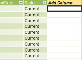
Illustration 15: Click the Top Row in the Column Labeled “Add Column”
- Select the function button (“fx”) to the left of the formula bar next.
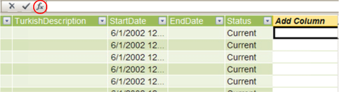
Illustration 16: Select the Function (fx) Button
The Insert Function dialog appears.
- Click the downward pointing arrow on the selector appearing atop the dialog under the Select a category label.
The following DAX function categories appear:
- All
- Date & Time
- Math & Trig
- Statistical
- Text
- Logical
- Filter
- Information
- Parent-Child
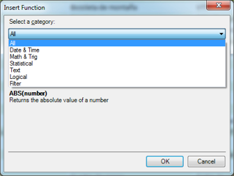
Illustration 17: Insert Function Dialog with Expanded Category Selector
- Select the Logical category.
- In the Select a function list that populates for the Logical category, select the IF() function, as shown in Illustration 18.
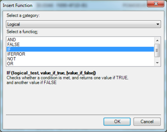
Illustration 18: Select the IF() Function
- Click OK to confirm the selection and dismiss the Insert Function dialog.
The IF keyword, proceeded by the “=” operator and followed by a left parenthesis ( “(“ ), appears in the formula bar, with a function usage tooltip appearing just underneath the function.
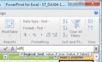
Illustration 19: The Beginning of the IF() Function, along with Tooltip, Appears
Because we need now to add a test of whether the column upon which we are focused, ProductLine, is blank, we will put ISBLANK() to work at this stage.
- Begin to type “ISBLANK()” into the formula bar, noting that AutoComplete immediately presents us with a list of functions, with ISBLANK() at the top, from which to select (once at least “IS” has been entered), as shown.
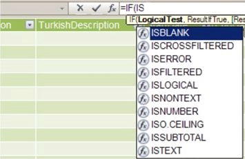
Illustration 20: Table as Suggested by AutoComplete
- Double-click ISBLANK in the dropdown menu to insert the function into the formula bar.
- Following the left parenthesis inserted by our selection of ISBLANK, type in the word “Product.”
- Scroll down and select Product[ProductLine] within the dropdown list to double-click / select the column, as depicted in Illustration 21.
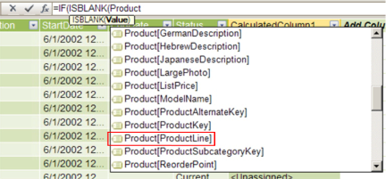
Illustration 21: Select the Product[ProductLine]Column
- Once the selector is dismissed, and =IF(ISBLANK(Product[ProductLine] appears in the formula bar, type (or copy and paste) the following syntax to the right:
), "<Unassigned>", Product[ProductLine]
The syntax, at this point, should be as shown here:
=IF(ISBLANK(Product[ProductLine]), "<Unassigned>", Product[ProductLine])
At this stage, the calculation is saying “if the Product Line is blank (the logical test), return ‘<Unassigned>.’ If a Product Line is specified, return that same Product Line.” The completed formula appears within the formula bar as shown:
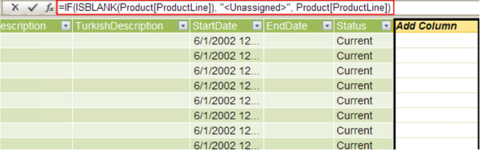
Illustration 22: The Completed Formula Appears
- Press the Enter key.
The column updates to reflect the action of the new calculation. Comparing this column to the original ProductLine column, we can verify that the value shown in the populated rows appears to be correct. (We could, of course, easily drag the new calculated column to the immediate right of the ProductLine column to facilitate easy comparison.)
Let’s name the column to distinguish it from the column upon which it is based, at this juncture.
- Right-click the new column header label (currently at its default of “CalculatedColumn1”), and select Rename Column from the cascading menu that appears.
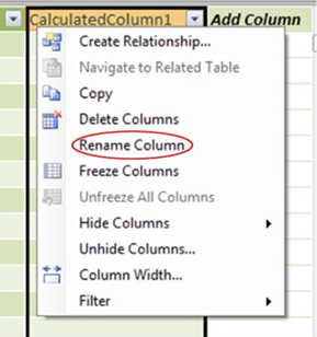
Illustration 23: Renaming the Column to its Ultimate Name
- Name the newly added column “Product Line Name” to provide a unique label.
The newly named column, with updated formula results, appears as partially depicted below.
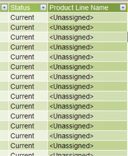
Illustration 24: The Results Appear in Each Row of the New Column (Partial View)
We thus see how we can employ ISBLANK() to reach a desired end, the renaming of a blank value, within the context of the prohibition against changing data directly in the PowerPivot data sheet view. In addition to rearranging the column to be beside the ProductLine column upon which it is based, we might also want to hide the base column to eliminate confusion, from the perspective of PivotTable operators using this PowerPivot source.
In the section that follows, we will access the PowerPivot calculated column we have created within a PivotTable. Moreover, we will get some hands-on exposure to putting the DAX ISBLANK() function to work within a calculated measure we will create in the PivotTable.
PivotTable Measure
In its most fundamental and common use, PowerPivot exists, as we have noted throughout the Stairway to PowerPivot and DAX series, to act as a data source for PivotTables. In this section, we will work further with the DAX function we have exposed in the PowerPivot calculated column section above, except this time, we will present values and calculations within a PivotTable.
We can begin our work with a PivotTable from either the Excel workbook or from the PowerPivot window. Because we’re already in the latter, we will proceed from there by taking the following steps:
- From the Product tab in the PowerPivot window, click the downward pointing arrow on the PivotTable button to cause the drop-down menu to appear, as shown.
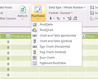
Illustration 25: The PowerPivot PivotTable Drop-down Menu Appears
While we will work with examples, at various times throughout our series, of some of the other options we see in the dropdown menu, we will build a single PivotTable in this session, and most of the practice sessions, of our series, as this will be the most straightforward (and rapid) avenue to getting hands-on exposure to the underlying PowerPivot data and DAX, in general.
- Click PivotTable in the dropdown menu we’ve exposed (the top selection).
We are returned to the Excel worksheet, where we encounter the Create PivotTable dialog.
- Ensure that the radio button labeled New Worksheet is selected.
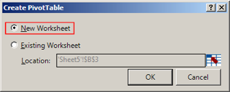
Illustration 26: Ensure the New Worksheet Option is Selected
- Click OK to accept the setting and dismiss the dialog.
The PivotTable placeholder / canvas, together with the PowerPivot Field List, appear on the new worksheet as depicted (compressed view):
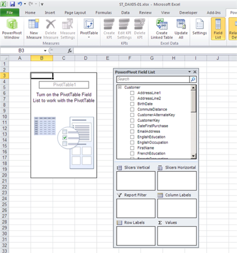
Illustration 27: The PivotTable Canvas Appears on the New Worksheet (Compressed View)
We’ll leave the placement of the new PivotTable at default.
NOTE: Because we cover the details for the first time in an earlier Level of the series, and particularly for those not already familiar with standard Excel PivotTables, Table 1 of Level 2: The DAX COUNTROWS() and FILTER() Functions, in the Accessing PowerPivot Calculated Columns from a PivotTable and Introducing Calculated Measures section gives a description for each of the areas / zones on the PowerPivot Field List. Other PivotTable basics are discussed there as well.
To gain some exposure to the use of the DAX ISBLANK() function within the PivotTable, we will replicate some of the steps we took with regard to the Product table, upon which we operated in the PowerPivot window in the earlier part of this Level. In accomplishing this, we’ll see how to approach what we did with the calculated column earlier, but this time we’ll do so with a calculated measure in the PivotTable. Moreover, we will touch upon more PivotTable – specific considerations as we encounter them. But first, we will pull the calculation we created earlier into a new PivotTable we construct, to allow us to see the output of our calculation when we select it from the PowerPivot Field List.
- Collapse the Customer table (expanded by default) in the Field List by clicking the “-” sign to its immediate left.
- Expand the Product table in the Field List by clicking the “+” sign to its immediate left.
The columns of the table, with which we worked in the PowerPivot window in the section above, appear as partially shown here:
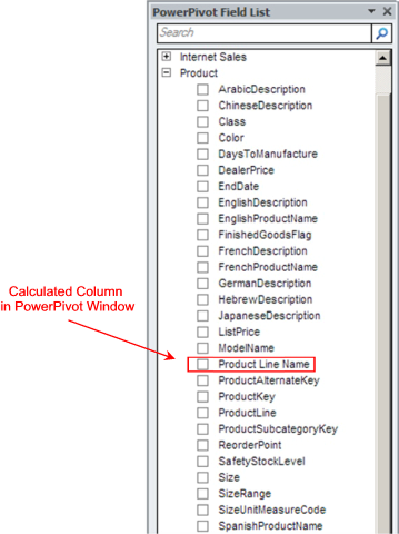
Illustration 28: Product Table in the PowerPivot Field List, Expanded to Show Fields
The highlighted field in the expanded list, of course, represents the calculated column that we created, and within which we employed the DAX ISBLANK() function, in the PowerPivot window earlier. We will pull this calculation into our new PivotTable like any other field at this point, and replicate (except with a different measure, Internet Sales Amount) the summary view with which our client colleagues illustrated the initial business requirement.
- Within the PowerPivot Field List, inside the expanded Product table, scroll to the Product Line Name column (which represents our new calculated column).
- Click the check box to the immediate left of the Product Line Name column.
Clicking the check box places the selected column, by default, into the Row Labels drop zone of the PivotTable.
- Within the Field List, collapse the Product table by clicking the “-” sign to its immediate left.
- Expand the Internet Sales table (appearing just above the Product table we have collapsed) in the Field List by clicking the “+” sign to its immediate left.
- Within the PowerPivot Field List, inside the expanded Internet Sales table, scroll to the SalesAmount column.
- Click the check box to the immediate left of the SalesAmount column.
Since the selected column is, in this instance, a numeric value, clicking the check box places it, by default, into the Values drop zone of the PivotTable.
The PowerPivot Fields List appears, with our two additions, as depicted in Illustration 29.
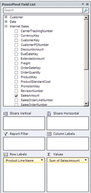
Illustration 29: Creating a New PivotTable with PowerPivot Data
The PivotTable summary we have constructed to this point appears as shown:
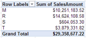
Illustration 30: PivotTable Summary with Internet Sales Data
We note that the summary above does not display any data with an unassigned Product Line. Let’s see how adding data from another fact table, Reseller Sales (and, hence, another line of the Adventure Works business) changes that.
- Within the Field List, once again, collapse the Internet Sales table.
- Expand the Reseller Sales table (appearing at the bottom of the Field List).
- Scroll to the SalesAmount column inside the expanded Reseller Sales table.
- Click the check box to the immediate left of the SalesAmount column.
The Reseller Sales Amount, another numeric value, appears within the Values drop zone of the PivotTable, underneath the Sales Amount values for Internet Sales.
- Within the Values drop zone of the Field List, right click the uppermost value (currently labeled “Sum of SalesAmount”).
- Select Edit Measure at the bottom of the context menu that appears, as depicted in Illustration 31.
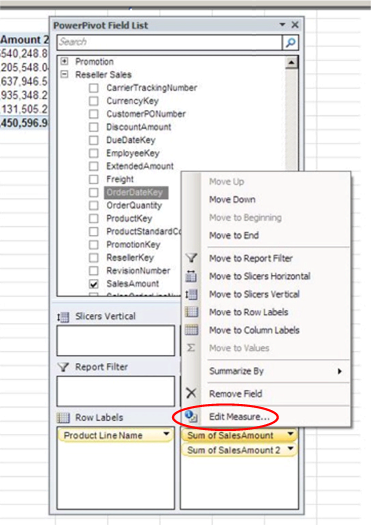
Illustration 31: Click Edit Measure
The Measure Settings dialog opens.
- Modify the text in the Custom Name box to “Internet Sales Amount,” as shown.
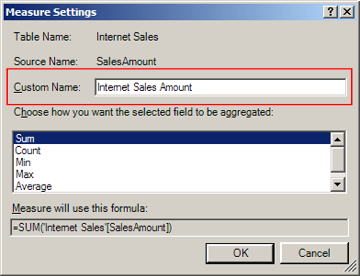
Illustration 32: Renaming the Measure
- Click OK to save the name change.
- Following the steps taken for the top “Sum of Sales Amount,” rename the second value, currently labeled “Sum of Sales Amount 2,” to “Reseller Sales Amount.”
The PowerPivot Field List drop zones appear, with our changes, as depicted below:
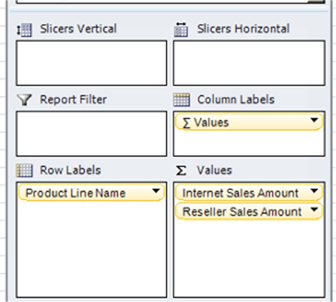
Illustration 33: The Field List Drop Zones, with Our Modifications
The PivotTable summary appears, with the measure we have added, as shown:
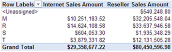
Illustration 34: PivotTable Summary with Added Reseller Sales Amount
This time, we note that the <Unassigned> product line appears. We can surmise that the Reseller Sales line of the business contains products that have no assigned product lines (an examination of the underlying data bears this out), as we might expect from the summary above.
The requirement of our client colleagues to see “Unassigned,” versus an empty label, in scenarios where the product line is empty has been met. This not only means less ambiguity for report readers / analysts with regard to the nature of the once-empty classification. Moreover, we have also added value from a user-friendliness perspective by leveraging the fact that the bracket character precedes both a number and letter in a standard sort; thanks to this, the unassigned portion of the summary will appear at the top of the labels list anytime the PivotTable is opened.
As a last consideration, let’s examine the use of the ISBLANK() function in a new calculated measure we will create within another PivotTable.
Having ascertained that we have met the last client need in an understandable manner, we ask if there is else with which we can assist. One of the group presents us with another small summary, comparing total Internet Sales and Reseller Sales, by Promotion, over all operating years contained in the current Adventure Works cube. The summary appears as depicted below.
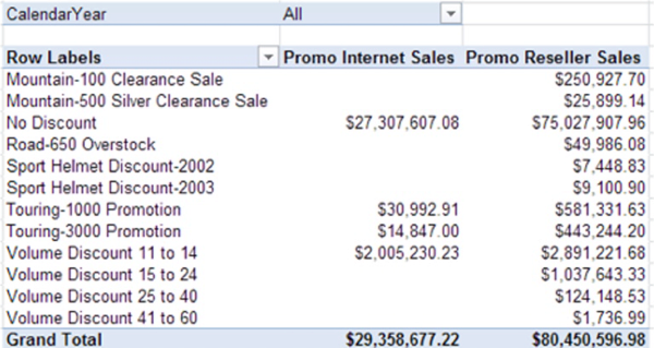
Illustration 35: Initial Summary Analysis, Promotions for Two Sales Types
The client representative tells us that he wishes to create a calculation that presents a ratio of promotion – driven Internet Sales to promotion – driven Reseller Sales. For those promotions that drove Reseller Sales, but resulted in no Internet Sales, he simply wants to indicate “NA,” rather than to show a zero, an empty cell, or some other potentially confusing result.
We recognize this as another opportunity to demonstrate the use of the DAX ISBLANK() function, and set about recreating the summary with which we have been presented in a PivotTable, within which we can then create a calculated measure to meet the stated business requirement.
- Click the PowerPivot tab atop the worksheet upon which we have completed our practice steps to this point, if necessary, to expose the related ribbon.
- Click the PivotTable button, as shown.
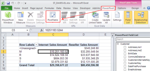
Illustration 36: Create Another PivotTable from the Current Position
The Create PivotTable dialog appears, once again.
- Ensure that the radio button labeled New Worksheet is selected, as we did in our earlier exercise.

Illustration 37: Ensure the New Worksheet Option is Selected, Once Again
- Click OK to accept the setting and dismiss the dialog.
The PivotTable placeholder / canvas, together with the PowerPivot Field List, appear on the new worksheet, as before. We’ll leave the placement of the new PivotTable at default, once again, as we recreate the initial summary view that our client colleague has presented.
- Collapse the Customer table (expanded by default) in the Field List by clicking the “-” sign to its immediate left.
- Expand the Promotion table in the Field List by clicking the “+” sign to its immediate left.
- Inside the expanded Promotion table, scroll to the EnglishPromotionName column.
- Click the check box to the immediate left of the EnglishPromotionName column.
Clicking the check box places the selected column, by default, into the Row Labels drop zone of the PivotTable. We see the Promotion Names appear within the rows axis of the PivotTable.
- Within the PowerPivot Field List, collapse the Promotion table by clicking the “-” sign to its immediate left.
- Expand the Internet Sales table in the Field List by clicking the “+” sign to its immediate left.
- Within the Field List, inside the expanded Internet Sales table, scroll to the SalesAmount column.
- Click the check box to the immediate left of the SalesAmount column.
Since the selected column is, in this instance, a numeric value, clicking the check box places it, by default, into the Values drop zone of the PivotTable, as we noted in our similar steps earlier.
- Within the Field List, collapse the Internet Sales table by clicking the “-” sign to its immediate left.
- Expand the Reseller Sales table in the Field List by clicking the “+” sign to its immediate left.
- Within the PowerPivot Field List, inside the expanded Reseller Sales table, scroll to the SalesAmount column.
- Click the check box to the immediate left of the SalesAmount column.
Clicking the check box places the corresponding column into the Values drop zone of the PivotTable, just below the identically named column we selected from the Internet Sales table earlier.
The Values drop zone of the PowerPivot Fields List appears, with our two additions, as depicted in Illustration 38.
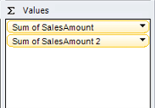
Illustration 38: Initial Appearance of Our Selections within the Values Drop Zone
Let’s take the opportunity to rename the Sales Amounts in a way that associates each with its respective parent table.
- Right-click the top value in the drop zone, currently entitled “Sum of Sales Amount.”
- Select Edit Measure at the bottom of the context menu that appears, as we did in the earlier exercise.
The Measure Settings dialog opens.
- Modify the text in the Custom Name box to “Promo Internet Sales” as shown.
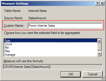
Illustration 39: Renaming the Measure
- Click OK to save the name change.
- Following the steps taken for the top “Sum of SalesAmount,” rename the second value, currently labeled “Sum of SalesAmount 2,” to “Promo Reseller Sales.”
Finally, although the simple summary presented by the client representative was for “all time in the cube,” as no Date filter was specified, we will give the information consumers that will be using the new summary the capability to filter upon calendar year(s), simply to demonstrate how this might be accomplished.
- Within the Field List, collapse the Reseller Sales table by clicking the “-” sign to its immediate left.
- Expand the Date table in the Field List by clicking the “+” sign to its immediate left.
- Within the PowerPivot Field List, inside the expanded Date table, scroll to the CalendarYear column.
- Drag the CalendarYear column to the Report Filter drop zone of the Field List.
CalendarYear now appears within the Report Filter drop zone of the Field List. Moreover, a filter selector is now readily accessible by prospective information consumers, just above the PivotTable.
The new PivotTable, together with corresponding PowerPivot Field List drop zones, appears as depicted below:
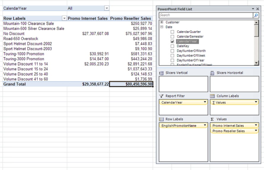
Illustration 40: The New Pivot Table and Field List Drop Zones
Having replicated the “starting position” that our client colleagues have presented, we are ready to add a calculation to the recipe. The purpose of the calculation, we recall, is to generate a ratio of promotion – driven Internet Sales to promotion – driven Reseller Sales. Moreover, an additional requirement has been described: that those promotions that drove Reseller Sales, but resulted in no Internet Sales, be indicated by a simple “NA,” rather than the more “natural” zero, empty cell, or other potentially ambiguous result. It is this latter requirement that affords us the opportunity to employ ISBLANK(), once again.
Let’s wrap up our example via the addition of the needed calculation, by taking the following steps:
- Return to the PowerPivot tab, if necessary, from the worksheet containing our current PivotTable.
- Click the New Measure button in the ribbon atop the tab (to the right of the PowerPivot Window button in the upper left of the ribbon), as shown:
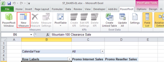
Illustration 41: Click the New Measure Button
The Measure Settings dialog appears.
- Select Reseller Sales in the dropdown selector labeled Table name atop the dialog.
- Type (or copy and paste) the following into both the Measure Name and Custom Name boxes of the dialog.
IS - RS Ratio
- Click the function button (“fx”) to the right of the Formula label, above the Formula input box of the dialog.
The Insert Function dialog appears.
- Leave the Select a category label at the default setting of “All” this time.
- Scroll, within the Select a function dropdown, to the IF function.
- Select the IF function, once again, as depicted in Illustration 42.
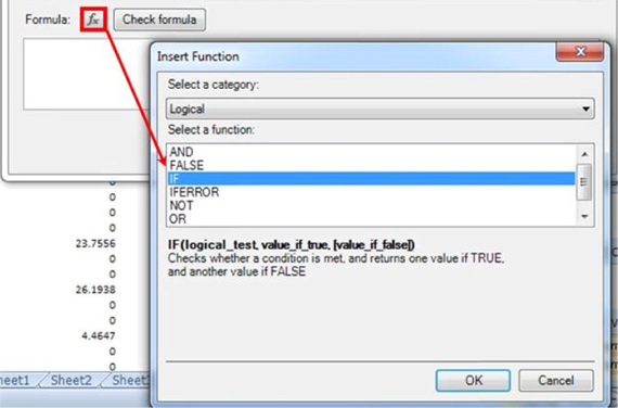
Illustration 42: Creating the New Ratio Measure
- Click OK to confirm the selection and dismiss the Insert Function dialog.
The IF keyword, proceeded by the “=” operator, and followed by a left parenthesis, once again, appears in the Formula input box of the Measure Settings dialog.
- To the immediate right of the left parenthesis (that appears to the right of the IF keyword), begin to type in the ISBLANK() function.
As we begin to type the function name, AutoComplete again presents us with a list of selections that begin with IS, and with which we will become familiar throughout progressive Levels of this series.
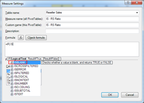
Illustration 43: Functions as Suggested by AutoComplete
- Within the Formula input box, continue to type “Internet“ after “ISBLANK( “ appears, until the Internet Sales table selections appear.
- Select ‘Internet Sales'[SalesAmount] from the dropdown selector, as shown.
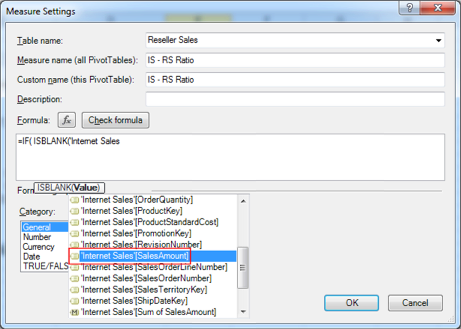
Illustration 44: Selecting the Desired Table Column
- Be sure to add a right parenthesis ( “ ) “ ) character, as shown below, after ‘Internet Sales'[SalesAmount].
The Formula input box should contain the following string, at this stage:
=IF(ISBLANK('Internet Sales'[SalesAmount])
- Once the selector is dismissed, and the above string appears, type the following syntax to its immediate right:
, BLANK(),
The formula string appears in the formula input box, at this stage, as shown.
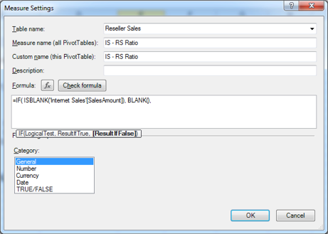
Illustration 45: The Formula Input Box with Formula at this Stage
At this point in creating the calculated column, our calculation is stating that, if the logical test (“Internet Sales.SalesAmount is blank”) is true, return a blank. Next, we need to add the value to return if the logical test is false.
- Type the following syntax to the right of the existing expression within the formula input box of the Measure Settings dialog:
'Internet Sales'[SalesAmount]/'Reseller Sales'[SalesAmount])
The formula string now appears, within the formula input box, as depicted.
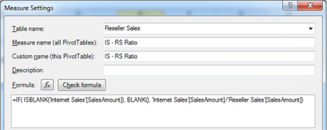
Illustration 46: The Text in the Formula Input Box
The formula string replicates the string we used in creating the somewhat similar calculated column in the PowerPivot window earlier.
- Click the Check formula button.
An error message is returned, as shown in Illustration 47.
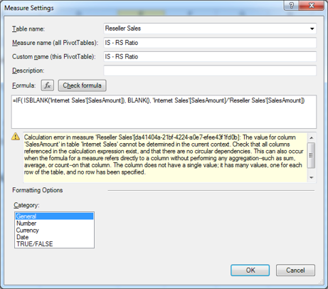
Illustration 47: An Error Regarding Context is Returned
The message indicates that “the value for column 'Sales Amount' in table 'Internet Sales' cannot be determined in the current context.” It becomes apparent, then, that a calculation that works at the row level, as we saw in our earlier example within the calculated column of the PowerPivot window, fails to generate the correct values in the PivotTable.
What we need, in fact, to do, as we have seen at similar junctures within other articles of the Stairway to PowerPivot and DAX series, is to pay attention to context. The idea, of course, is to perform the calculation, via our new measure, at the cell level of the new PivotTable and not at the row level of the PowerPivot window. In this case, we must generate the desired value by calculating a ratio that divides the total of 'Internet Sales'[SalesAmount] by the total of 'Reseller Sales'[SalesAmount].
Having attempted to use the same general DAX approach that we employed at the PowerPivot level, only to have received the context error noted, let’s go back and make a couple of minor modifications to our measure. These modifications relate, again, to the concept of context (via the SUM() function) in the PivotTable.
- Modify the syntax currently within the formula input box of the Measure Settings dialog, to place each occurrence of 'Internet Sales'[SalesAmount] and 'Reseller Sales'[SalesAmount] within the SUM() function. In other words, modify the existing syntax within the input box from this:
=IF(ISBLANK('Internet Sales'[SalesAmount]), BLANK(),
   'Internet Sales'[SalesAmount]/'Reseller Sales'[SalesAmount])
… to this:
=IF(ISBLANK( SUM('Internet Sales'[SalesAmount])), BLANK(),
   SUM('Internet Sales'[SalesAmount]) / SUM('Reseller Sales'[SalesAmount]))
The completed formula string appears, within the formula input box, as depicted.
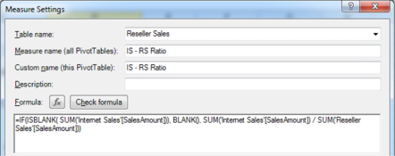
Illustration 48: The Complete, Modified Text in the Formula Input Box
- Click the Check formula button, once again.
The message returned this time indicates “no errors in formula,” as shown in Illustration 49.
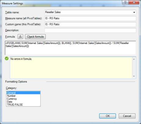
Illustration 49: “No Errors in Formula” is Indicated
We’re close to wrapping this measure up and observing its operation. To finish, let’s format the output of our calculation to meet the preference of many accounting and finance professionals, in general. We’ll format the new ratio as a percentage, with a single decimal point.
- Click the Number option within the Category selector (lower left corner of the Measure Settings dialog).
- Select Percentage within the Format selector that appears, among other context-sensitive settings, to the right of the Category selector.
- Select “1” in the Decimal places “dialer.”
The context-sensitive settings in the Formatting Options section of the Measure Settings dialog appear, with our settings, as depicted.
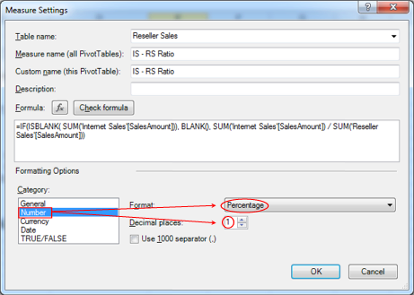
Illustration 50: Formatting Options in the Measures Setting Dialog
- Click the OK button to accept our changes, and to dismiss the Measure Settings dialog.
The dialog box disappears, and the newly calculated measure appears in a column on the right side of our PivotTable. Let’s take a look at the data to ascertain that the values generated by the new measure appear in the expected way.
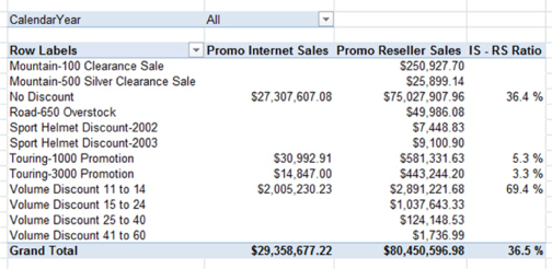
Illustration 51: The New Measure Appears as Expected
It’s relatively easy to see that our new ratio calculation appears to return the correct percentage values row-by-row in the individual lines we see above, or the blanks that we have conditionally specified as appropriate (that is, where Internet Sales is empty). Moreover, we note that the ratio behaves as desired in the “Grand Total” line – generating the proper ratio between the two columns concerned (Promo Internet Sales / Promo Reseller Sales), instead of simply totaling the rows above. Therefore it appears safe to conclude that the PivotTable performs in a complete and accurate manner, with respect to operation upon aggregations of data as defined by the context of the current cell.
Summary
In this Level of the Stairway to PowerPivot and DAX series, we exposed the DAX ISBLANK(), and revisited the DAX BLANK(), functions. We discussed the general purposes and operation of ISBLANK(), and then focused upon using ISBLANK() in general, as well as the illustrating ways ISBLANK() can be employed, particularly in situations where we can combine it with other functions, to achieve a result similar to something we might need to generate for clients or employers in our own environments.
As part of our exploration, we examined the syntax surrounding ISBLANK(), undertaking a couple of illustrative examples of the uses of the function in practice exercises, and then exploring the results datasets we obtained in the practice examples. We worked with the combination of ISBLANK() and other functions to deliver illustrative answers to business questions, within both a PowerPivot calculated column and a PivotTable calculated measure we built in the section that followed. As we put each calculation to use within the PivotTable, we compared and contrasted the values returned by each, explaining the reasons behind their differences, and discussing considerations in choosing which of these two calculation approaches to take in meeting business requirements in our own environments.