

In my first article about Data Mining we talked about Data Mining with a classical example named AdventureWorks. In this example I am going to complement the first article and talk about the decision trees. Let me resume in few words how the Data Mining model worked.
The data mining is an expert system. It learns from the experience. The experience can be obtained from a table, a view or a cube. In our example the data mining model learned from the view named dbo.vtargetmail. That view contained the user information about the customer.
People usually think that they need to use cubes to work with Data Mining. We worked with the Business Intelligence Development Studio or the SQL Server Data Tools (in SQL 2012), but we did not use cubes, dimensions or hierarchies (we could use it, but it is not mandatory). We simply used a view.
If we run the following query we will notice that we have 18484 rows in the view used.
Select count(1) from dbo.vtargetmail
Something important to point about Data Mining is that we need a lot of data to predict the future. If we have few rows in the view, the Mining Model will be inaccurate. The more data you have, the more accurate the model will be.
Another problem in data mining is the input of data for the data mining. How can we determine which information is important for the Mining Model? We can guess a little bit.
Let´s return to the Adventureworks Company and let´s think about the customers that may want to buy bikes. The salary may be important to buy a bike. If you do not have money to buy a bike, you will not buy it. The number of cars is important as well. If you have 5 cars you may not want to have a bike because you prefer to drive your cars.
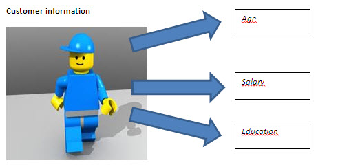
There are some data that may be useful as the input to predict if the customer is going to buy a bike or not. How can we determine which columns of data are important or which ones are not? In order to start, we can think about it. Is it important for the model the address or the email of the customers?
It may not be important, especially the email. Does someone with Hotmail have less chances to buy a bike that a person with Gmail? I guess not. They are some input data that we could remove from the model intuitively. However the Data Mining tool lets you determine which columns affect or not the decision to buy or not a new bike.
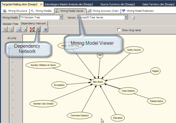
The Dependency Network
In the Data Mining Model, go to the Mining Model Viewer Tab. In the Model Viewer Tab, go to the Dependency Network Tab. The Bike Buyer Oval is the Analysis that we are doing. We want to analyze if a person X is a possible buyer. The number of Children, Yearly Income, Region and the other variables are the columns of the view. With the Dependency Network, we can analyze which column has influence to buy or not a Bike.
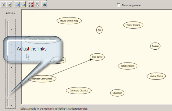
If you adjust the link bar, you can define which column has more influence to buy or not a bike.
In this example the number of cars owned is the most important factor to buy or not a Bike.
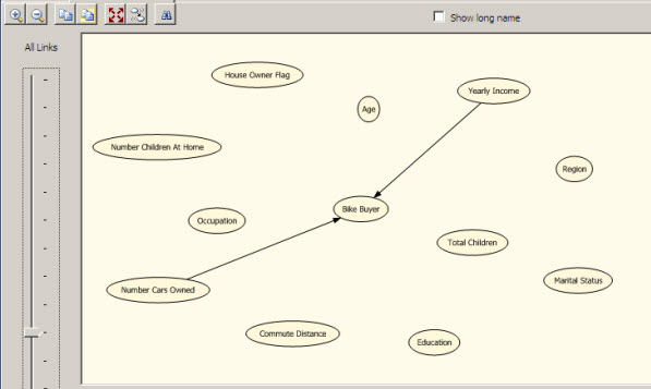
The second factor to buy a bike is the Yearly Income. This information is very important for Business Analysts and the marketing team.
In my first article we used Decision Trees. Decision Trees are one of the different algorithms used by Microsoft to predict the future. In this case to predict if a customer x is going to buy a bike or not. In the viewer combo box we can select the option Microsoft Generic Content Tree Viewer. This option let you get some technical details about the algorithm.
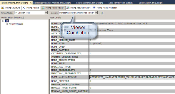
For more information about NODES, cardinality visit this link: http://msdn.microsoft.com/en-us/library/cc645772(v=110).aspx
About Decision Trees
Decision trees are the first basic algorithm that we used in this article. This Data Mining Algorithm divides the population used to predict if the customers want to buy or not a bike in different nodes. The nodes have branches and child nodes.
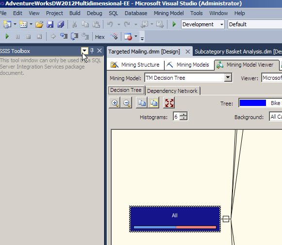
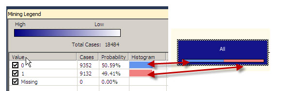
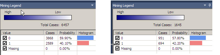
The first node contains all the cases. If you click on the node, there is a Mining legend at the right with all the cases used. The value 0 is the number of customers that did not buy the bikes. The value 1 is the group of user that bought bikes. There are colors to graphically see the percentages of users of each category.
The second node divides the cases in the number of cars owned.
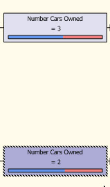
You can see that the colors of the node are different. The darker nodes contain more cases, if you click in the Number Cars Owned=2 you will notice that the number of cases is 6457. If you click in the Number Cars Owned=3, the number of cases is 1645.
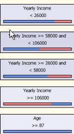
The other nodes are related to the Yearly Income and Age. There is a lot of information that can be analyzed here.
I am going to talk about the Mining accuracy chart in future articles. To end this article, we are going to have a list of prospective buyers and predict if they will buy or not a bike.
For this example, we are going to use the table dbo.Prospectivebuyers table that is included in the AdventureWorksDW database. Let’s move to the Mining Model Prediction Tab.
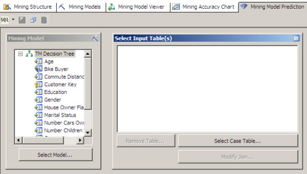
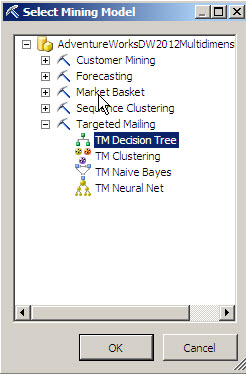
Let’s select a Model. In this case, select the Decision Tree.
In the select Input Table(s) click the Select Case Table.
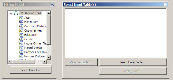
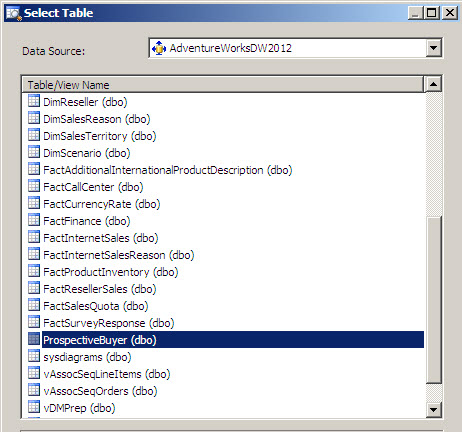
In the select Table Windows, select the ProspectiveBuyer Table. This table contains all the Prospective Buyers. We are going to determine the probability to buy or not bikes.
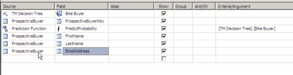
In the source select the TM Decision Tree. Also select the following fields from the ProspectiveBuyer:
ProspectivebuyerKey, firstName, lastname and Email. Finally select a Prediction Function and select the PredictProbability.
What we are doing is to show the firstname, lastname, email and the probability to buy a bike. The PredictProbability shows a value from 0 to 1. The closer the value goes to 1, the closer the user will buy a bike.
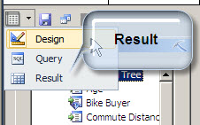
To verify the results, select the result option
Now you have the information of the prospective buyes and the probability to buy bikes. You predict the future again!
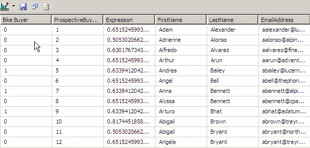
For Example Adam Alexander has a probability to buy of 65 % while Adrienne Alonso has a probability of 50 %. We should focus on the guys with more probabilities and find why do they prefer to buy bikes. The main reason is the number of cars and after that the year income.
Conclusion
In this article we talked a little more about Data Mining and then we explained how the decision tree worked. Finally we predict the future with a list of possible customers and found which have more probability to buy bikes.