

Background
We have recently been working on large data migration project for one of our clients and thought I would share how Delayed Durability helped us overcome a performance issue when the solution was moved to the client’s Development domain.
I won’t go into details of the project or the finer detail of our proposed solution as I have plans to put some more content together for that but in short the migration of the data was to be run by a (large) number of BIML generated SSIS (Child) packages for each table to be migrated, derived from a meta data driven framework with each stage being run by a master package, all of which run by a MasterOfMaster packages.
To maximize throughput, utilise as much processing power as possible, reduce the time it would take to run the migration and control the flow we built a series of sequence containers each running it’s own collection of Child Packages. We built the framework in such a way that these could be run in parallel or linear and each master package could contain as many containers (no pun intended) of child packages as required. This also allowed us to handle the order that packages were run in, especially those with dependencies whilst keeping the potential for parallelising (is that a word? No idea but I like it) the whole process as much as possible. Leaving the MaxConcurrentExecutables property to -1 mean’t we could push the processing to run up to 10 packages at once due to the VM having 8 cores (on Integration, 4 cores on Development) and this value of -1 allows the maximum number of concurrently running executables to equal the number of processors plus two.
An small example of how the MasterOfMaster and a Master Package for a stage looked is shown below:
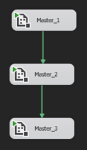
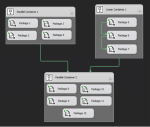
Each container number could have Parallel and/or Linear Containers and both must succeed before the next Container level can start.
NOTE that this is just an example representation, naming conventions shown do not reflect the actual solution.
Problem
During development and initial testing on our own hardware, we had the migration at the time running at ~25minutes for around 600 packages (ie. tables) covering (what we termed) RawSource–>Source–>Staging which was well within the performance requirements for the stage that development was at and for what was initially set out. The rest of this blog post will hone in specifically on Source–>Staging only.
However, once we transferred the solution to the clients development environment things took a turn for the worse. In our environment we were running VMs with 8 cores, 16GB RAM and utlising SSDs. The client environment was running SQL Server 2016 Enterprise on VMWare vSphere 5.5, 8 vCPUs, 32GB RAM (for Integration, Development was half this) but the infrastructure team have done everything in their power to force all VMs onto the lower tier (ie. slow disks) of their 3-PAR SAN and throttle them in every way possible, just to make things more of a challenge. Even though the VM’s themselves were throttled we were confident that we wouldn’t see too much of a performance impact, especially as this was only a subset of the processing to be done so we needed it to be quick and it will only ever get longer and longer.
How wrong we were. On the first run the processing (for Source–>Staging) took around 141 minutes, yes you read that right, a full 116 minutes longer than the whole process took on our hardware! Wowza, didn’t see that one coming. I won’t delve too much into the investigations as again that will be saved for another blog post but essentially we were seeing a huge amount of the WRITELOG wait type since moving to the client environment. We believed the reason for this was due to the significant amount of parallel processing (running of SSIS packages in parallel loading to the same DB) we were doing and the SAN didn’t seem to be able to handle it. One other thing to note, due to truncations not being flagged as error’s in OLE DB Destination fast load data mode access, some of the packages that weren’t a direct copy where we knew the schema was exactly the same were run in non-fast load, ie row-by-row which puts additional stress on the system as a whole.
I will be blogging at a later date regarding how we managed to get everything running in fast load and handle the truncation via automated testing instead.
Solution
Enter Delayed Durability.
I won’t enter into too much detail regarding what this is or how it specifically works as this has been blogged by many others (Paul Randal, Aaron Bertrand to name just a couple) but my favourite description of delayed durability is comes from the msdn blogs and they refer to it as a “lazy commit“. Before you ask, yes we understood the issues of implementing such a change but the migration process was always a full drop and reload of the data so we didn’t care if we lost anything as we could simply run the process again.
Setting delayed durability at the database level we were able to control which Databases involved in the process we wished to have this without altering the BIML framework or code itself to handle it at the transaction level. By simply applying this to the Source and Staging databases we reduced the processing time from 141 minutes to 59 minutes. This wasn’t exactly perfect but shaving more than half the time off with one simple change and pushing the WRITELOG wait stat way way down the list was a great start.
As a side not, we have managed to get the processing from ~59mins to ~30mins without changing the VM/hardware configuration but I will leave that for another post.
Proof
When I first set out with this blog post it was only going to be a few paragraphs giving an insight into what we did however, I thought that all this would be pointless without some visualisation of the processing both before and after.
Row-by-Row with no Delayed Durability
We needed to get a baseline and where better to start than capturing the metrics through SentryOne and using Adam Mechanic’s spWhoIsActive we can see what I was talking about with the WRITELOG wait stat:
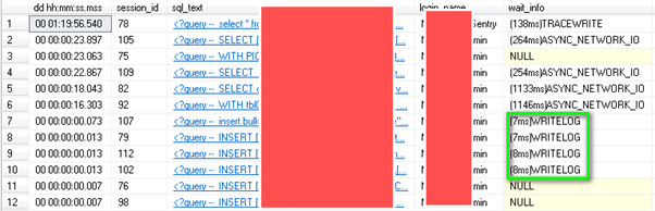
Granted the wait time themselves was relatively low, these were apparent almost every time we hit F5 and running our wait stat scripts in was in the top 3. A sample of the processing indicating this wait stat can also be seen below:
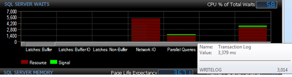
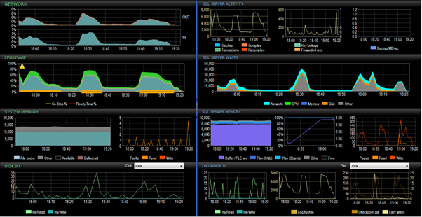
As stated previously, overall the Source–>Staging process took 141 minutes and the overall processing from SentryOne PA was captured:
Row-by-Row with Delayed Durability
So when we ran the same process with Delayed Durability we can see straight away that the transactions/sec ramp up from ~7000 to ~12500. Top left shows without Delayed Durability, bottom left with Delayed Durability and right shows them side by side:
![]()
![]()
![]()
The overall process for Source–>Staging took only 59 minutes. I’ve tried to capture the before/after in the image below, the highlighted section being the process running with Delayed Durability forced:
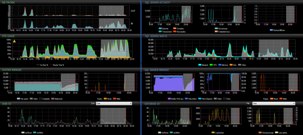
You can see from this the drastic increase in Transactions/sec and reduction in Log Flushes.
Two package execution time examples (trust me that they are the same package) showing that with Delayed Durability the processing time was only 43% (166sec down to 72sec and 991sec to 424sec) ) of that without Delayed Durability set. Apologies for the poor image quality….
![]()
![]()
To me that is a huge reduction for such a simple change!
Conclusion
So should you go out and apply this to all your production databases right this second? No, of course you shouldn’t. We applied this change for to fix a very specific problem in an isolated environment and were willing to take the hit on losing data if the server crashed – are you, or more importantly your company willing to lose that data? I’m taking an educated guess that this will be a no but for certain situations and environments this configuration could prove to be very useful.
Links
- https://msdn.microsoft.com/en-gb/library/dn449490.aspx
- http://www.sqlskills.com/blogs/paul/delayed-durability-sql-server-2014/
- https://sqlperformance.com/2014/04/io-subsystem/delayed-durability-in-sql-server-2014
- ……or use you preffered search engine and search for “SQL Server delayed durability”
- https://msdn.microsoft.com/en-us/library/microsoft.sqlserver.dts.runtime.package.maxconcurrentexecutables.aspx
