Supervised training of an artificial neural network entails training the network to associate defined patterns with specified labels. Optical Character Recognition is an example of supervised training, where each input pattern is mapped to an alphanumeric character.

In unsupervised training, a neural network learns to extract recurring patterns from noisy data. One of the earliest practical applications of unsupervised artificial neural network learning was performed by the United States Navy, where neural networks were trained to recognize underwater sounds and those sounds were empirically mapped to classes of watercraft and marine animals.

The Mathematics of an Artificial Neural Network

Mathematically, a neural network is a set of simultaneous nonlinear equations with an infinite set of acceptable solutions, the fundamental mathematical component of which is the neuron.

A neuron accepts one or more input signals through connections to other neurons or outside stimuli and transforms their sum into an output signal. The sum of the input signals can range from negative to positive infinity. The output (activation) signal can range from zero to one. The most common mathematical transformation function used to emulate a biological neuron activation signal is the sigmoid function:

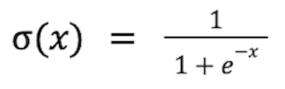
When using the sigmoid function to calculate the activation signal of a neuron, the variable x is replaced with the sum of the input signals.

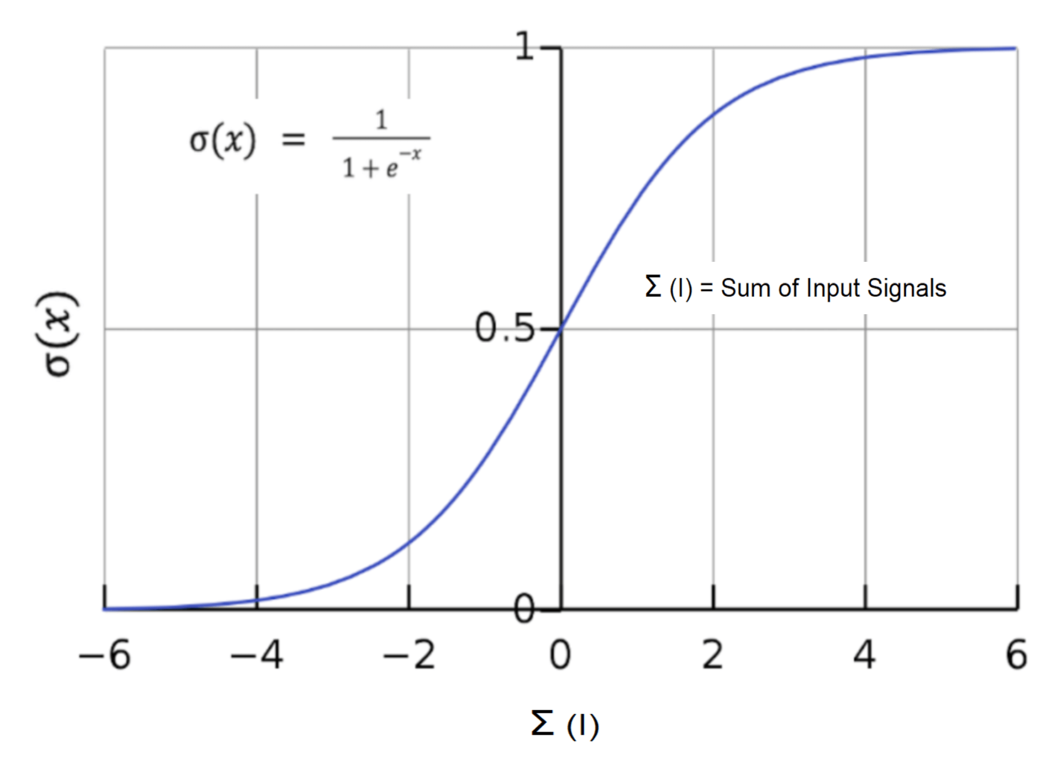
This graph of the sigmoid function displays the sum of the input signals on the x-axis and the resulting output activation signal on the y-axis.

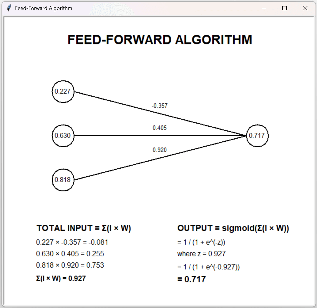
The Feed-Forward Algorithm: Calculating the Activation Value of a Neuron

In the illustration below, three input neurons of varying activation magnitudes I are connected to an output neuron via connections of varying weighting factors W to yield an activation signal in the output neuron that is computed using the sigmoid function.

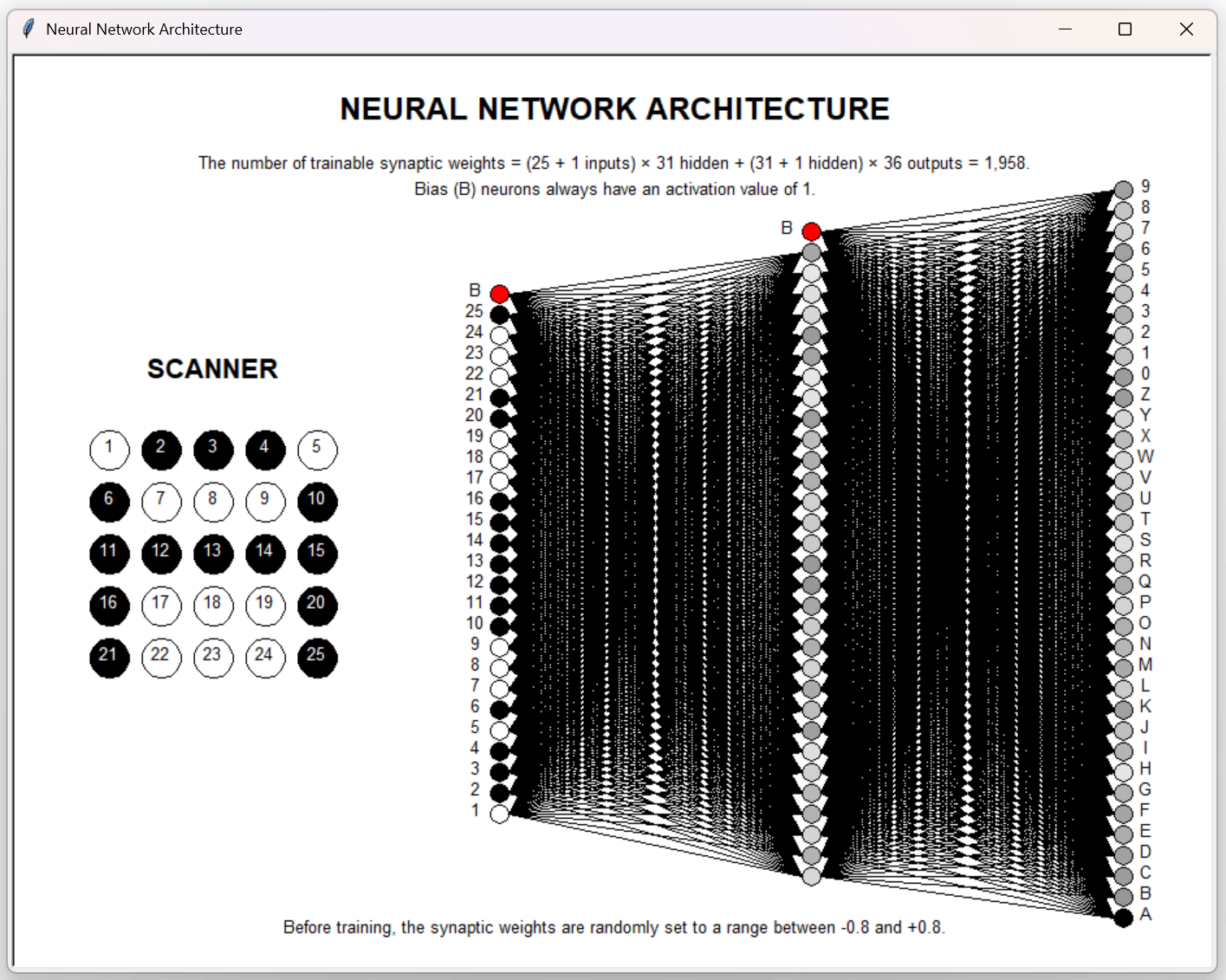
Artificial Neural Network Architecture

The most common artificial neural network design consists of three layers of neurons: an input layer, a middle hidden layer, and an output layer. The first two layers also contain a bias neuron, a neuron which has a constant activation value of one. Each neuron in an upper layer is connected to each neuron in the succeeding layer. The number of neurons to configure in the middle layer is commonly determined by adding the number of neurons in the input layer and output layer and dividing by two. Before training begins, each of the connection weights is randomly set within the range -0.8 to +0.8.

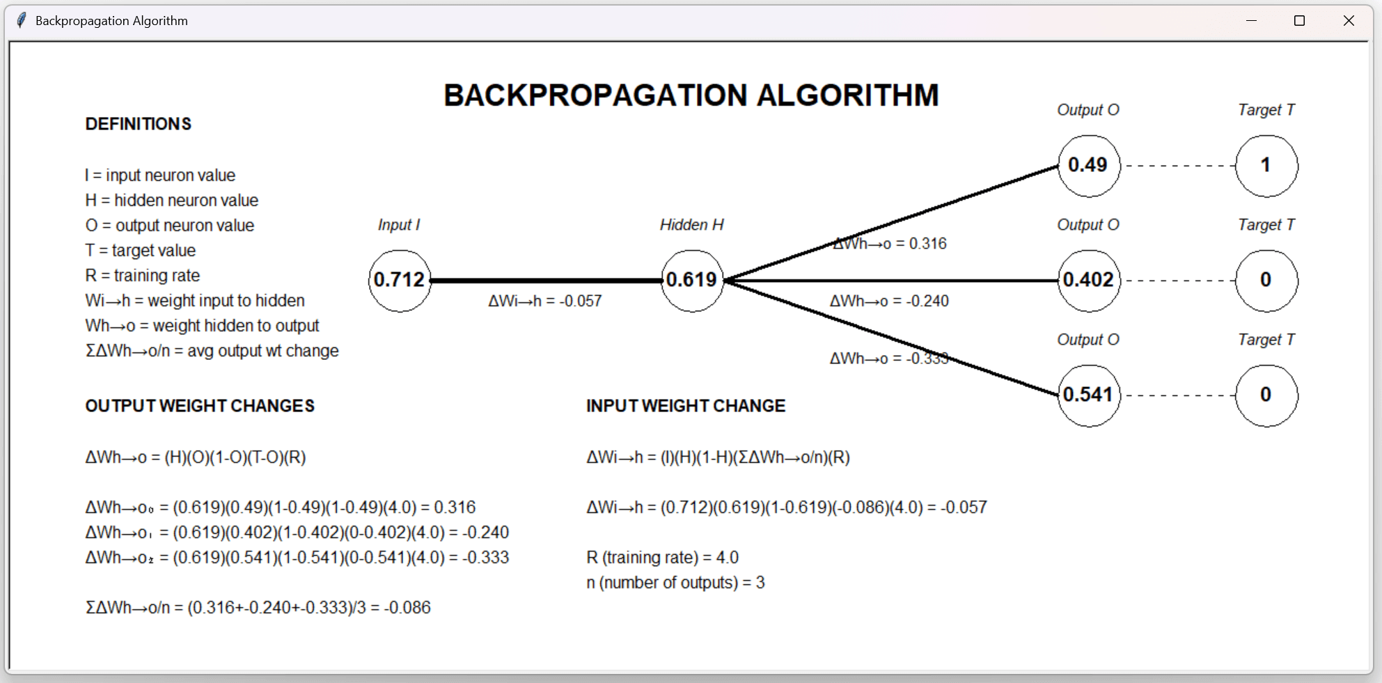
The Back-Propagation Algorithm: Calculating the Correction Factors of Network Connection Weights

After a pattern is fed from the input neurons to the output neurons, the error for each output neuron is calculated by subtracting the neurons activation value from its target value for that pattern. The weights connecting the neuron layers are then increased or decreased in proportion to the quantity of their contribution to the error. A positive error results in addition of a correction value to a connection weight, while a negative error results in subtraction of a correction value from a connection weight.

The image below illustrates calculation of the weight changes in both layers of connections.

Supervised Training Demo

Execute the OCR app from the github repository: https://github.com/CodeSkink/TrainingDemos/releases.

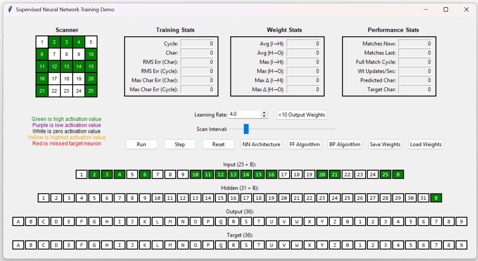
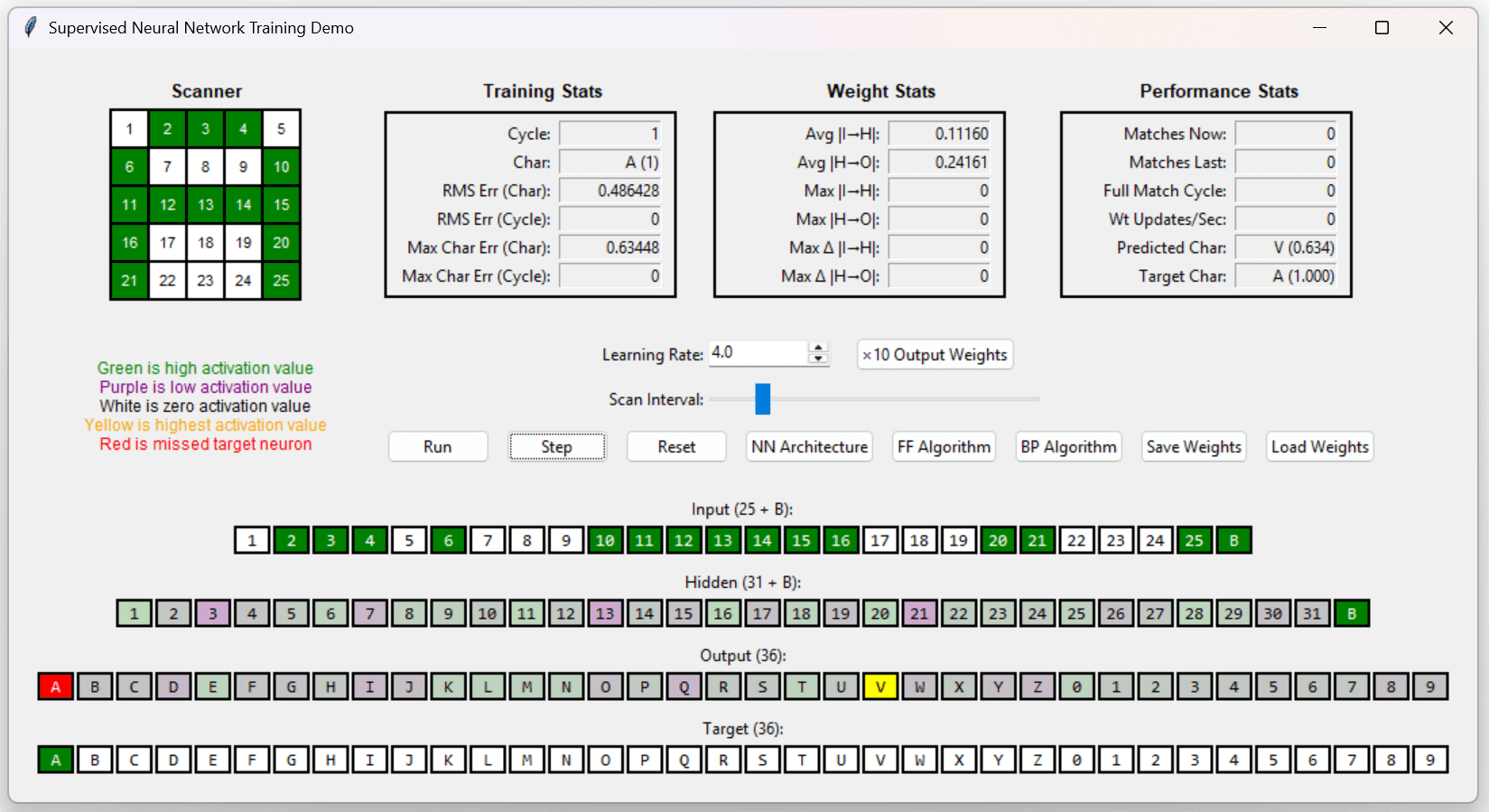
When the “Step” button of the OCR app is clicked, the first training pattern is scanned.

Clicking the “Run” button causes the app to cycle through 36 training patterns. On the first cycle where all 36 patterns are recognized, the cycle number will be inserted into the “Full Match Cycle” text box while the app continues to train.

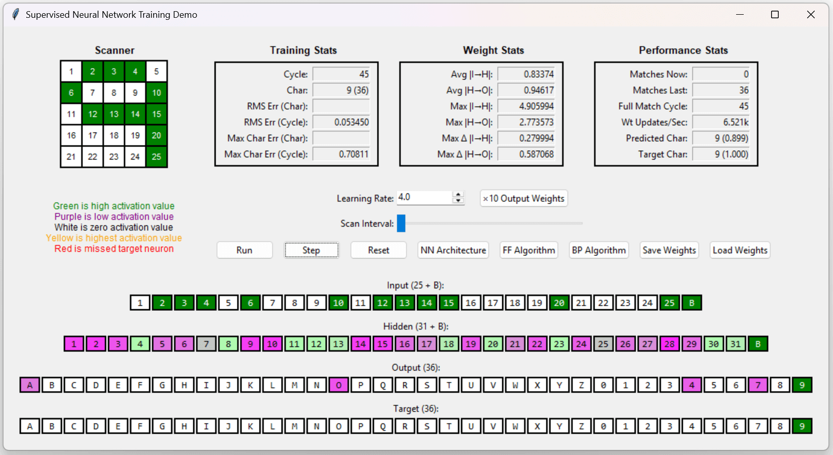
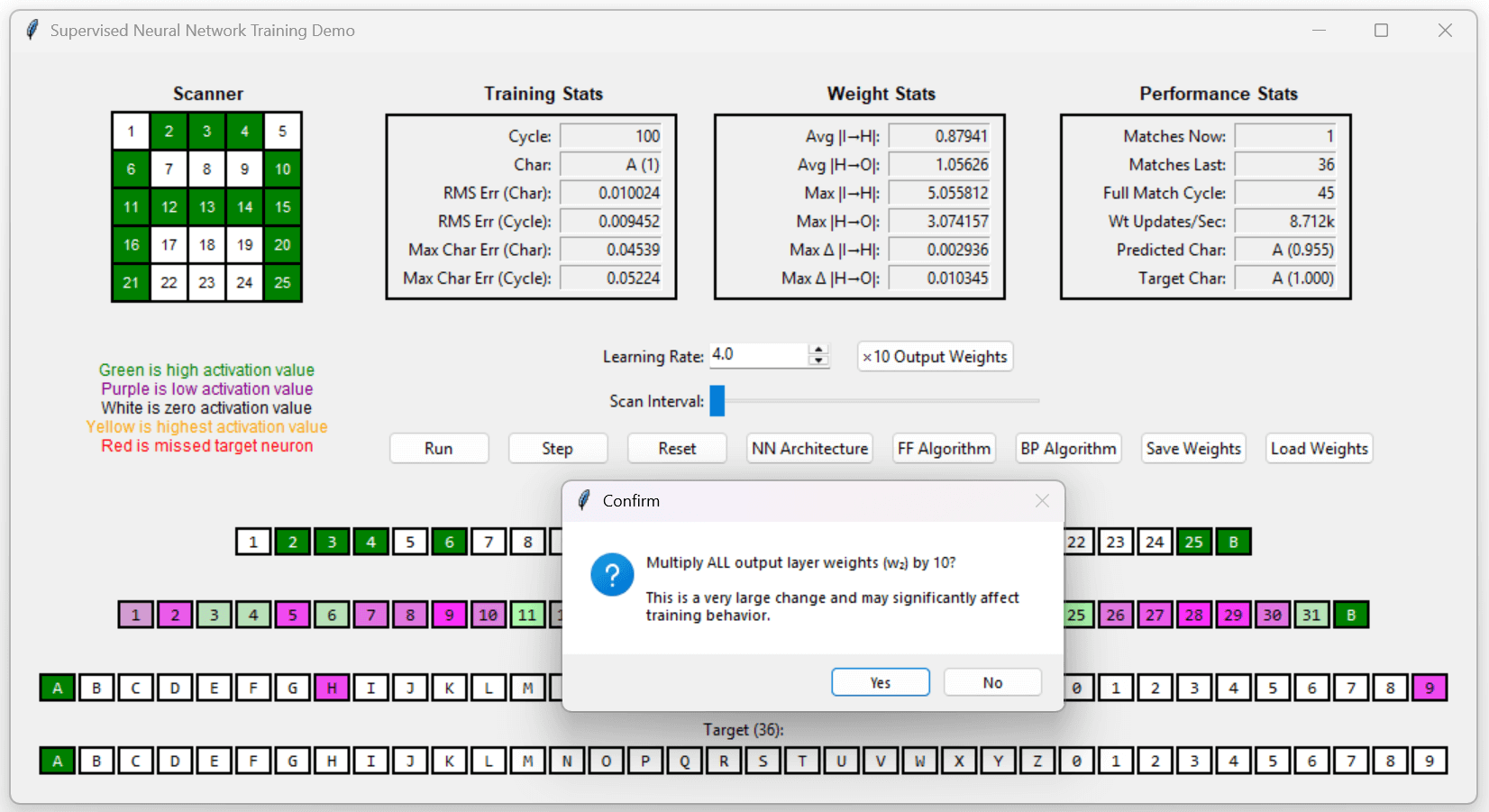
After the network recognizes all 36 training patterns, clicking the “x 10 Output Weights” button will multiply all the output weights by ten, causing the error status fields to go to zero, or close to it.

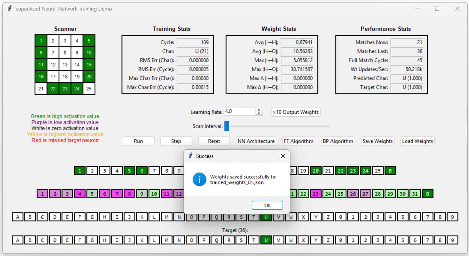
Clicking the “Save Weights” button allows a set of trained weights to be saved for future use by clicking the “Load Weights” button.

Unsupervised Training Demos

Execute the autoencoder app from the GitHub repository.

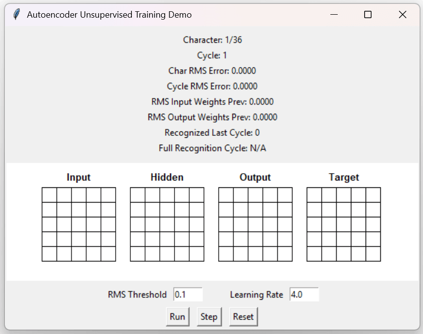
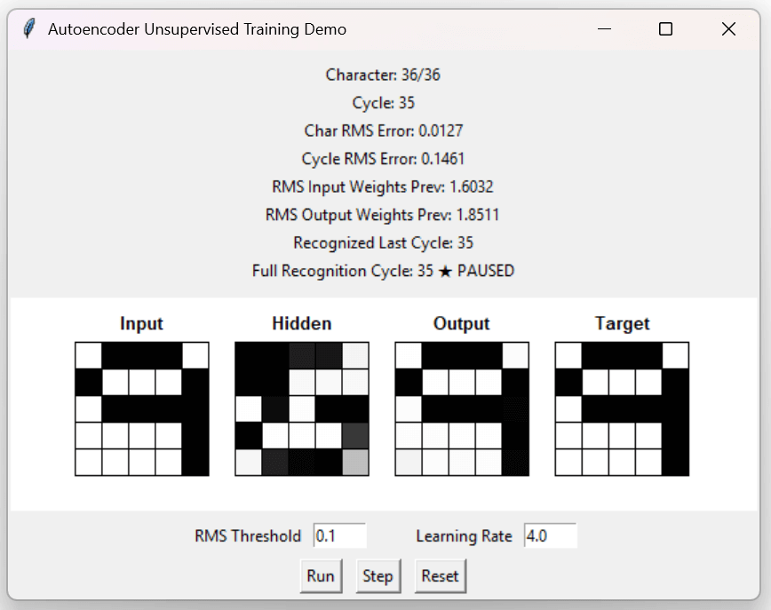
This app cycles through the same 36 training patterns as the supervised app, but the target pattern is the same as the input pattern. Click the “Step” button to display the first training and target patterns.

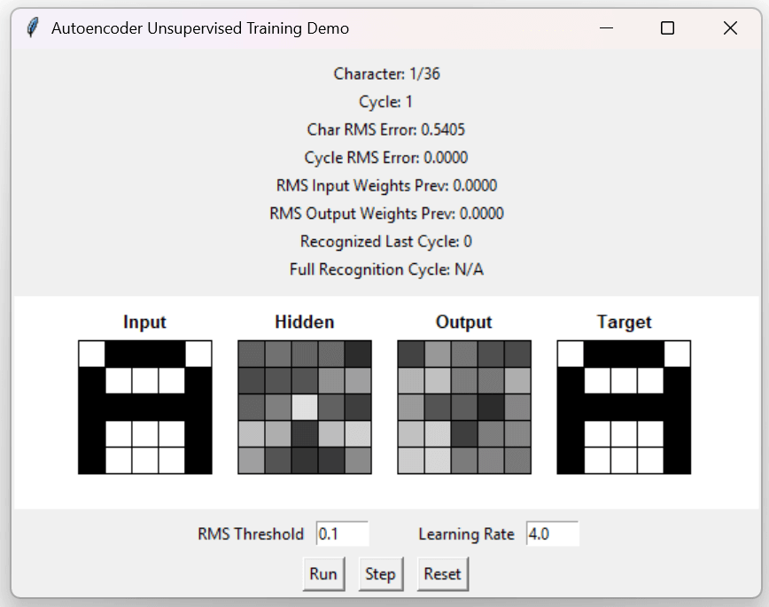
Click the "Run" button. When all 36 output patterns match the input patterns, training is complete.

Noisy Autoencoder

Execute the noisy_autoencoder app from the GitHub repository.

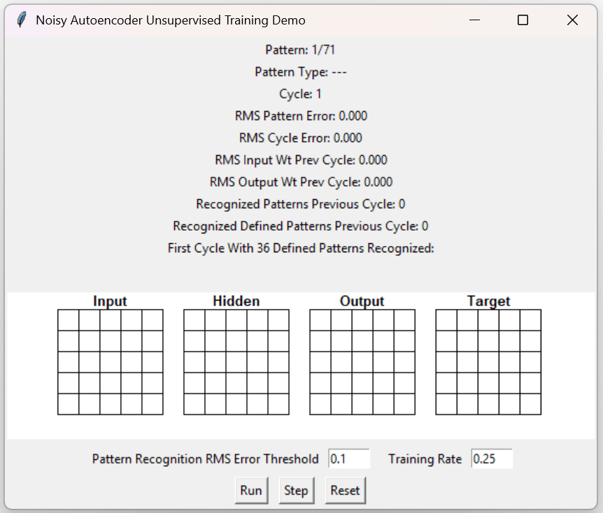
This app trains on the same set of 36 input patterns as the autoencoder app, but interleaved between each defined pattern is a random pattern. The set of random patterns is refreshed at the end of each training cycle. Click the “Step” button twice to see the first random pattern.

Click the "Run" button. Training is complete when all 36 defined patterns are recognized.

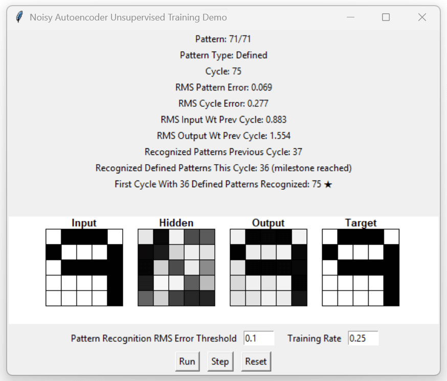
There is an anomaly, however. On the cycle previous to the cycle when 36 defined patterns were recognized, 37 total patterns were recognized. This means that at least two random patterns were erroneously determined to be recurring patterns. The next demo app illustrates a bigger anomaly than that.

Random Autoencoder

Execute the random_autoencoder app from the GitHub repository.

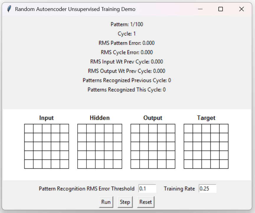
This app trains on a set of 100 random patterns per cycle, with 100 new random patterns generated at the end of each training cycle. Click the "Step" button to see the first random pattern.

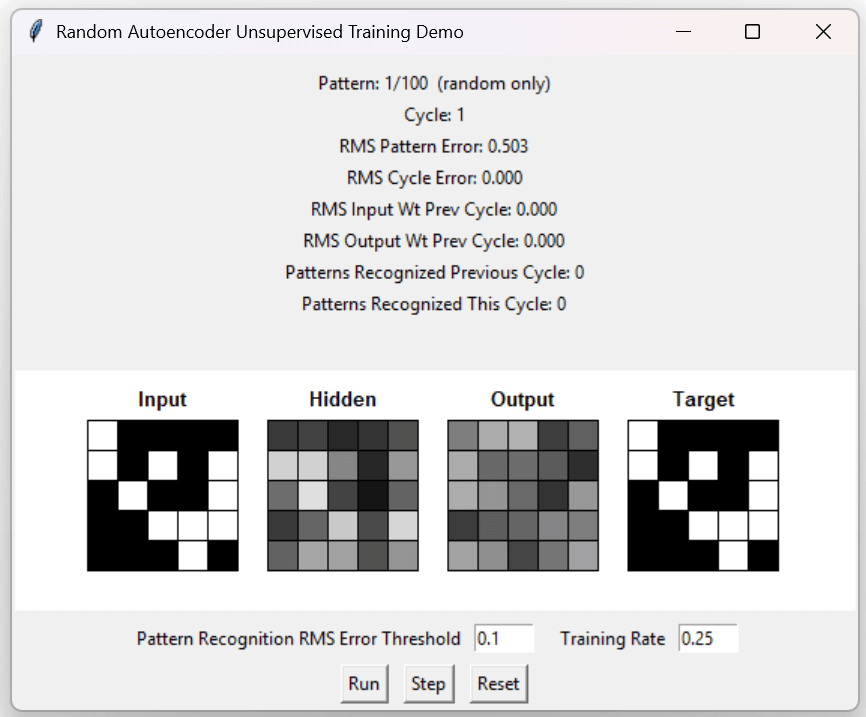
Click the "Run" button. Training is complete when 100 random patterns are recognized.

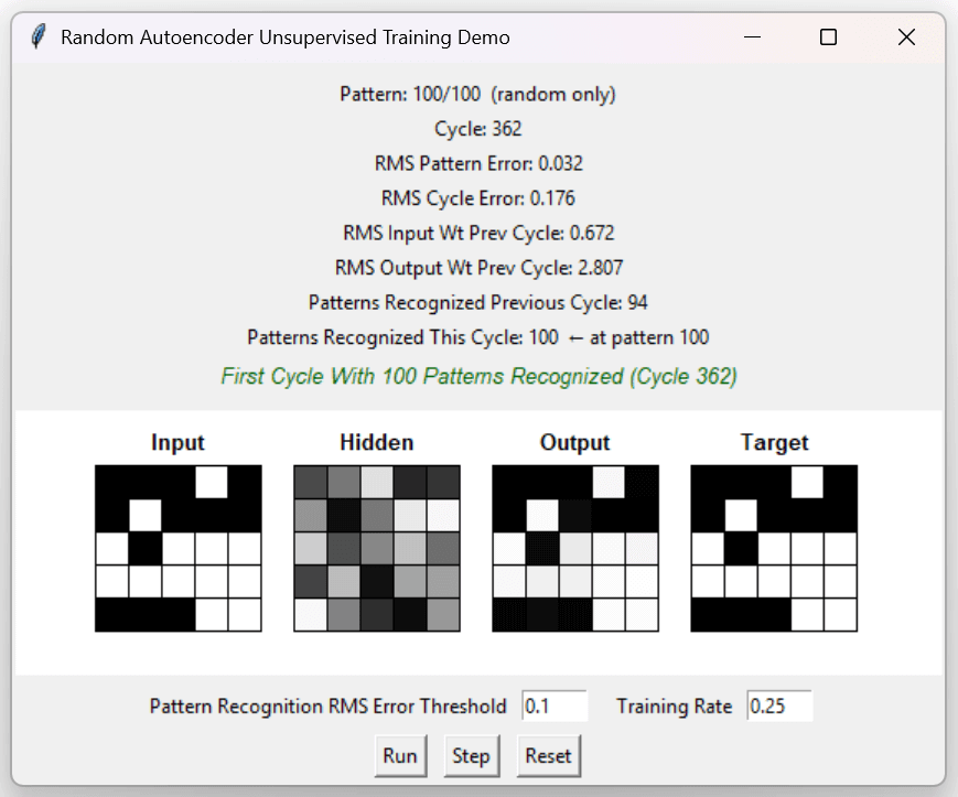
How can all 100 random patterns be recognized as recurring? A 5x5 grid of binary values can generate 2^25 = 33,554,432 possible patterns. After 362 cycles, the network has trained on 36,200 random patterns.

(100) x (36,200) / (33,554,432) = 0.11%

The neural network has only been exposed to 0.11% of possible patterns, but seems to recognize almost any pattern it scans. The explanation for this is that the neural network is no longer training on patterns. It is now training on individual neurons and has established a one-to-one relationship between each input neuron and its corresponding output neuron.

Conclusion

This article has demonstrated the mathematics of artificial neural networks, supervised and unsupervised modes of neural network training, and how unsupervised training can morph into mimicking patterns rather than recognizing them.

Source and Executable Code Link: https://github.com/CodeSkink/TrainingDemos/releases