Disk and CPU related performance counters and DMV information can be difficult to interpret and compare when activity levels differ massively. This Cellular Automation (CA) application places a precise workload that can be repeated, adjusted and measured. It includes various 'Pattern Generators', one that uses Geometry and places a CPU load, another that uses set based queries that are IO bound and another 'Hekaton' version that uses in-memory tables and compiled stored procedures. All three are implementations of 'Conway's Game of Life', and a precise way to benchmark and compare the relative performance of different SQL Servers. Data is inserted at the start of each benchmark then automated using a fixed set of rules, buffer pool pressure doesn't affect the benchmarks too heavily and typically, the same query plans are used regardless of SQL Server version or platform.
Benchmarking Process Overview
The following link explains the rules implemented by this application: http://en.wikipedia.org/wiki/Conway's_Game_of_Life . It is a Cellular Automation application with a virtual grid of z , y coordinates pre-populated with different patterns, the rules below are then applied and repeated. A cell represents a coordinate or a Merkle.
- Any live cell with fewer than two live neighbours dies, as if caused by under-population.
- Any live cell with two or three live neighbours lives on to the next generation.
- Any live cell with more than three live neighbours dies, as if by overcrowding.
- Any dead cell with exactly three live neighbours becomes a live cell, as if by reproduction.
The benchmarking procedure creates one of three initial patterns which are then 'automated' according to the rules above, the table below shows all parameters available:
| Parameter Name | Type | Description | Default |
| @Batches | INT | Number of calls to the benchmarking procedures | 0 |
| @CPU_Benchmark | BIT | Execute the CPU bound benchmark procedure | 0 |
| @IO_Benchmark | BIT | Execute the SQL Server IO bound benchmark procedure | 0 |
| @Hek_Benchmark | BIT | Execute the Hekaton in-memory, compiled benchmark procedure | 0 |
| @NewPatternsInBatch | INT | Number of new patterns (automations) generated by each call | 0 |
| @DisplayPatterns | BIT | Show final result pattern | 0 |
| @Initialize | BIT | Clear previous results for session before execution | 1 |
| @StressLevel | TINYINT | 1 = small oscillating initial pattern, 2 = intermediate oscillating initial pattern, 3 = Large and expanding initial pattern | 1 |
| @Description1 | VARCHAR | For later analysis | |
| @Description2 | VARCHAR | For later analysis | |
| @Description3 | VARCHAR | For later analysis |
Setup and Execution
Run the attached setup scripts in SQLCMD mode to create the CA Benchmark database, then call the CA_Benchmark procedure, set the 'Database Name', 'Data File' and 'Log File' variables before execution.
CPU Benchmarking Simulation - Geometry
With the 'CPU benchmark' parameter, the coordinates are converted to geometric polygons, cell sizes are increased by 20% and the geometric 'Intersect' method is used to count adjacent Merkles. This cell expansion is illustrated by the 'Toad' pattern (see wiki) shown below in its base state/starting pattern.

When the automation rules are applied to the pattern above, the pattern below is generated on the 1st iteration, it returns to it's base state/starting pattern on the next iteration, this simple Stress Level 1 pattern changes between 2 states.
To simulate this example, execute the T-SQL below against the CA database (top left pattern).
EXECUTE dbo.CA_Benchmark @IO_Benchmark = 1, @DisplayPatterns = 1 ,@StressLevel = 2, @Batches = 1, @NewPatternsInBatch = 1;
EXECUTE dbo.CA_Benchmark @IO_Benchmark = 1, @DisplayPatterns = 1 ,@StressLevel = 2, @Batches = 1, @NewPatternsInBatch = 2;
OLAP Bias Workload Simulation
The screenshot below shows the initial patterns created at Stress Level 3.

The screen shot below shows the patterns after 60 automations, 2 new 'Gosper Glider Guns' patterns (see Wiki) are created every 30th automation which increases the CPU, IO and memory cost. The more new patterns are generated, the more like an OLAP workload the automation benchmark becomes.

To simulate this example, execute the T-SQL below against the CA database.
EXECUTE dbo.CA_Benchmark @IO_Benchmark = 1, @DisplayPatterns = 1 ,@StressLevel = 3, @Batches = 1, @NewPatternsInBatch = 1;
EXECUTE dbo.CA_Benchmark @IO_Benchmark = 1, @DisplayPatterns = 1 ,@StressLevel = 3, @Batches = 1, @NewPatternsInBatch = 60;
Use Case Example - 'Max Degree of Parallelism' Settings
The CA benchmarking process was invoked using OSTRESS with the parameters below, MAXDOP was set to 0 for the first two benchmarks then to 1 for the next two.
| Concurrent Requests | @Batches | @IO_Benchmark | @NewPatternsInBatch | @StressLevel | @Description1 | @Description2 |
| 2 | 1000 | 1 | 1 | 1 | OLTP | MAXDOP=0 |
| 2 | 10 | 1 | 100 | 3 | OLAP | MAXDOP=0 |
| 2 | 1000 | 1 | 1 | 1 | OLTP | MAXDOP=1 |
| 2 | 10 | 1 | 100 | 3 | OLAP | MAXDOP=1 |
OLTP Bias Workload Results
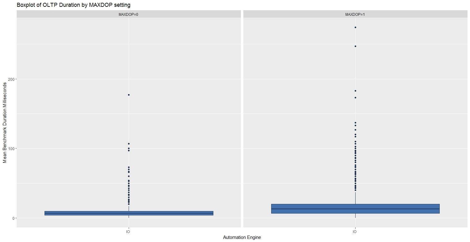
When processing 1,000 small batches, the benchmark typically completed in half the time with MAXDOP set to 0.
| Benchmark | Min. | 1st Qu | Median | Mean | 3rd Qu | Max |
| OLTP - MAXDOP=0 | 0.00 | 4.00 | 7.00 | 8.67 | 10.00 | 177.00 |
| OLTP - MAXDOP=1 | 0.00 | 7.00 | 13.00 | 17.87 | 20.00 | 274.00 |
OLAP Bias Workload Results
When processing 10 larger expensive batches, the benchmark typically completed in half the time with MAXDOP set to 1.
| Benchmark | Min. | 1st Qu | Median | Mean | 3rd Qu | Max |
| OLAP - MAXDOP=0 | 42,997 | 48,348 | 49,664 | 50,497 | 51,430 | 59,897 |
| OLAP - MAXDOP=1 | 19,580 | 22,020 | 23,488 | 23869 | 24,648 | 36,147 |

These graphs and statistics were produced using the R script below:
rm(list=ls())
ca <- read.csv(file = "c:/DataScience/CA_MAXDOP_20170930.csv", header = TRUE, sep = ",", stringsAsFactors = FALSE)

# Factors
ca$StartTime <- as.factor(ca$StartTime)
ca$AutomationEngine <- as.factor(ca$BenchmarkPerspective)
ca$OLTP_OLAP <- as.factor(ca$Description1)
ca$MAXDOP <- as.factor(ca$Description2)

#install.packages("ggplot2")
library("ggplot2")

fill <- "#4271AE"
line <- "#1F3552"

ca_OLTP <- subset(ca, ca$OLTP_OLAP == "OLTP")
ca_OLAP <- subset(ca, ca$OLTP_OLAP == "OLAP")

p1 <- ggplot(ca_OLTP, aes(x = AutomationEngine, y = BatchDurationMS)) + geom_boxplot()
p1 <- p1 + scale_x_discrete(name = "Automation Engine") +
  scale_y_continuous(name = "Mean Benchmark Duration Milliseconds") +
  geom_boxplot(fill = fill, colour = line)
p1 <- p1 +  ggtitle("Boxplot of OLTP Duration by MAXDOP setting")
p1 <- p1 + facet_wrap(~MAXDOP)
p1

p1 <- ggplot(ca_OLAP, aes(x = AutomationEngine, y = BatchDurationMS)) + geom_boxplot()
p1 <- p1 + scale_x_discrete(name = "Automation Engine") +
  scale_y_continuous(name = "Mean Benchmark Duration Milliseconds") +
  geom_boxplot(fill = fill, colour = line)
p1 <- p1 +  ggtitle("Boxplot of OLAP Duration by MAXDOP setting")
p1 <- p1 + facet_wrap(~MAXDOP)
p1

summary(subset(ca_OLTP$BatchDurationMS,ca_OLTP$MAXDOP== "MAXDOP=0"))
summary(subset(ca_OLTP$BatchDurationMS,ca_OLTP$MAXDOP == "MAXDOP=1"))
summary(subset(ca_OLAP$BatchDurationMS,ca_OLAP$MAXDOP== "MAXDOP=0"))
summary(subset(ca_OLAP$BatchDurationMS,ca_OLAP$MAXDOP == "MAXDOP=1"))
Use Case - Measuring the cost of an Extended Event session.
The CA benchmarking process was invoked using OSTRESS with the parameters below, the extended event session (see references) ON for the first two benchmarks then OFF for the next two.
| Concurrent Requests | @Batches | @IO_Benchmark | @NewPatternsInBatch | @StressLevel | @Description1 | @Description2 |
| 2 | 1000 | 1 | 1 | 1 | OLTP | XE OFF |
| 2 | 10 | 1 | 100 | 3 | OLAP | XE OFF |
| 2 | 1000 | 1 | 1 | 1 | OLTP | XE ON |
| 2 | 10 | 1 | 100 | 3 | OLAP | XE ON |
OLTP Bias Workload Results
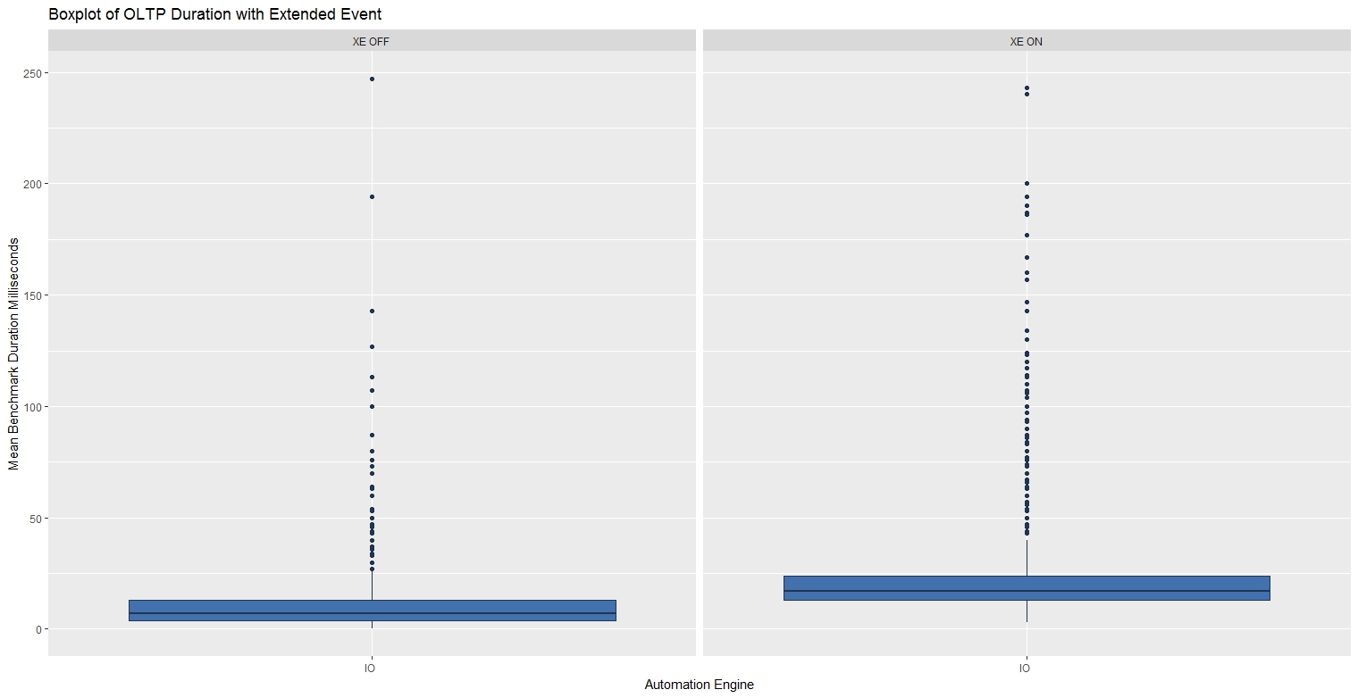
When processing 1,000 small batches with the XE Session running, the mean benchmark times roughly double.
| Benchmark | Min. | 1st Qu | Median | Mean | 3rd Qu | Max |
| OLTP - XE ON | 3.00 | 13.00 | 17.00 | 23.93 | 24.00 | 243.00 |
| OLTP - XE OFF | 0.00 | 4.00 | 7.00 | 10.00 | 13.00 | 247.00 |
OLAP Bias Workload Results
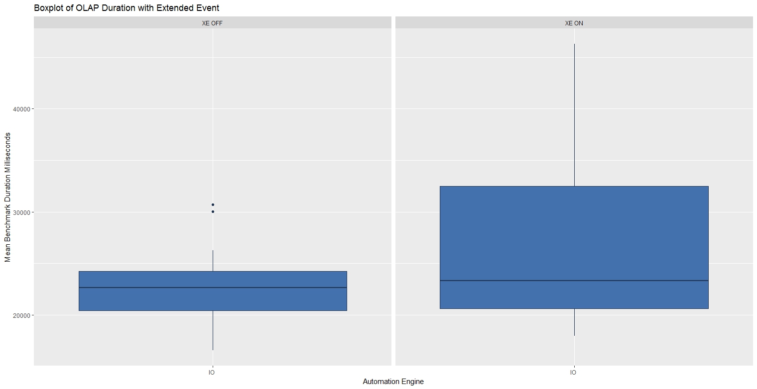
When processing 10 larger expensive batches with the XE Session running, there was far greater variability in the benchmark times.
| Benchmark | Min. | 1st Qu | Median | Mean | 3rd Qu | Max |
| OLAP - XE ON | 17,946 | 20,612 | 23,337 | 27,078 | 32,496 | 46,286 |
| OLAP - XE OFF | 16,540 | 20,433 | 22,652 | 22,773 | 24,252 | 30,703 |
These graphs and statistics were produced using the R script below:
rm(list=ls())
ca <- read.csv(file = "c:/DataScience/CA_XE_20170930.csv", header = TRUE, sep = ",", stringsAsFactors = FALSE)

# Factors
ca$StartTime <- as.factor(ca$StartTime)
ca$AutomationEngine <- as.factor(ca$BenchmarkPerspective)
ca$OLTP_OLAP <- as.factor(ca$Description1)
ca$XE <- as.factor(ca$Description2)

#install.packages("ggplot2")
library("ggplot2")

fill <- "#4271AE"
line <- "#1F3552"

ca_OLTP <- subset(ca, ca$OLTP_OLAP == "OLTP")
ca_OLAP <- subset(ca, ca$OLTP_OLAP == "OLAP")

p1 <- ggplot(ca_OLTP, aes(x = AutomationEngine, y = BatchDurationMS)) + geom_boxplot()
p1 <- p1 + scale_x_discrete(name = "Automation Engine") +
  scale_y_continuous(name = "Mean Benchmark Duration Milliseconds") +
  geom_boxplot(fill = fill, colour = line)
p1 <- p1 +  ggtitle("Boxplot of OLTP Duration with Extended Event")
p1 <- p1 + facet_wrap(~XE)
p1

p1 <- ggplot(ca_OLAP, aes(x = AutomationEngine, y = BatchDurationMS)) + geom_boxplot()
p1 <- p1 + scale_x_discrete(name = "Automation Engine") +
  scale_y_continuous(name = "Mean Benchmark Duration Milliseconds") +
  geom_boxplot(fill = fill, colour = line)
p1 <- p1 +  ggtitle("Boxplot of OLAP Duration with Extended Event")
p1 <- p1 + facet_wrap(~XE)

p1

summary(subset(ca_OLTP$BatchDurationMS,ca_OLTP$Description2 == "XE ON"))
summary(subset(ca_OLTP$BatchDurationMS,ca_OLTP$Description2 == "XE OFF"))
summary(subset(ca_OLAP$BatchDurationMS,ca_OLAP$Description2 == "XE ON"))
summary(subset(ca_OLAP$BatchDurationMS,ca_OLAP$Description2 == "XE OFF"))
Use Case - Hekaton Benchmark
A Microsoft whitepaper, 'In-Memory OLTP – Common Workload Patterns and Migration Considerations', highlights Hekaton performance and describes the workload patterns that suit in-memory OLTP. This is an independent assessment of Hekaton that includes the scripts and processes used so the result can be reproduced and is open to scrutiny.
Benchmarks were taken for OLTP and OLAP bias work loads running as a single request then again in two concurrent requests. This was an attempt to access the performance of in memory tables and compiled stored procedures on a Windows Server 2016 virtual machine with SQL Server 2016 SP1, 8 GB of RAM and 2 vCPU's. The CA benchmarking process was invoked using OSTRESS and the parameters below to simulate first an OLTP bias workload with many small batches, then an OLAP bias workload.
| Concurrent Requests | @Batches | @IO_Benchmark | @Hek_Benchmark | @NewPatternsInBatch | @StressLevel | @Description1 | @Description2 |
| 2 | 1000 | 1 | 0 | 1 | 1 | OLTP | Two Concurrent Requests |
| 2 | 1000 | 0 | 1 | 1 | 1 | OLTP | Two Concurrent Requests |
| 2 | 10 | 1 | 0 | 100 | 3 | OLAP | Two Concurrent Requests |
| 2 | 10 | 0 | 1 | 100 | 3 | OLAP | Two Concurrent Requests |
| 1 | 1000 | 1 | 0 | 1 | 1 | OLTP | One Concurrent Request |
| 1 | 1000 | 0 | 1 | 1 | 1 | OLTP | One Concurrent Request |
| 1 | 10 | 1 | 0 | 100 | 3 | OLAP | One Concurrent Request |
| 1 | 10 | 0 | 1 | 100 | 3 | OLAP | One Concurrent Request |
OLTP Bias Workload Results
When processing 1,000 small batches, Hekaton performance was typically four times faster and more consistent mainly due to precompiled stored procedures.
| Benchmark | Min. | 1st Qu | Median | Mean | 3rd Qu | Max |
| OLTP - SQL IO | 0.00 | 7.00 | 10.00 | 16.77 | 14.00 | 507.00 |
| OLTP - Hekaton | 0.00 | 3.00 | 3.00 | 3.81 | 4.00 | 217.00 |

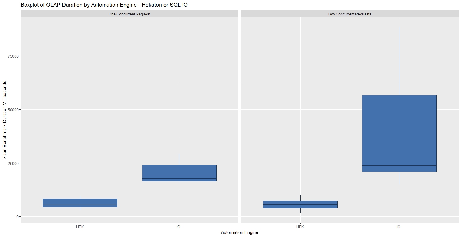
OLAP Bias Workload Results
When processing 10 larger batches, Hekaton performance was typically five times faster and far more consistent mainly due to lock and latch contention changes.
| Benchmark | Min. | 1st Qu | Median | Mean | 3rd Qu | Max |
| OLAP - SQL IO | 15,050 | 17,294 | 23,534 | 32,275 | 40,173 | 88,643 |
| OLAP - Helaton | 1,363 | 4,323 | 5,630 | 5,963 | 7,430 | 10,040 |
These graphs and statistics were produced using the R script below:
rm(list=ls())
ca <- read.csv(file = "c:/DataScience/CA_Hekaton_20170930.csv", header = TRUE, sep = ",", stringsAsFactors = FALSE)

# Factors
ca$StartTime <- as.factor(ca$StartTime)
ca$AutomationEngine <- as.factor(ca$BenchmarkPerspective)
ca$OLTP_OLAP <- as.factor(ca$Description1)
ca$Concurreny <- as.factor(ca$Description2)

#install.packages("ggplot2")
library("ggplot2")

fill <- "#4271AE"
line <- "#1F3552"

ca_OLTP <- subset(ca, ca$OLTP_OLAP == "OLTP")
ca_OLAP <- subset(ca, ca$OLTP_OLAP == "OLAP")

p1 <- ggplot(ca_OLTP, aes(x = AutomationEngine, y = BatchDurationMS)) + geom_boxplot()
p1 <- p1 + scale_x_discrete(name = "Automation Engine") +
  scale_y_continuous(name = "Mean Benchmark Duration Milliseconds") +
  geom_boxplot(fill = fill, colour = line)
p1 <- p1 +  ggtitle("Boxplot of OLTP Duration by Automation Engine - Hekaton or SQL IO")
p1 <- p1 + facet_wrap(~Concurreny)
p1

p1 <- ggplot(ca_OLAP, aes(x = AutomationEngine, y = BatchDurationMS)) + geom_boxplot()
p1 <- p1 + scale_x_discrete(name = "Automation Engine") +
  scale_y_continuous(name = "Mean Benchmark Duration Milliseconds") +
  geom_boxplot(fill = fill, colour = line)
p1 <- p1 +  ggtitle("Boxplot of OLAP Duration by Automation Engine - Hekaton or SQL IO")
p1 <- p1 + facet_wrap(~Concurreny)
p1

summary(subset(ca_OLTP$BatchDurationMS,ca_OLTP$AutomationEngine == "HEK" & ca_OLTP$Description2 == "One Concurrent Request"))
summary(subset(ca_OLTP$BatchDurationMS,ca_OLTP$AutomationEngine == "HEK" & ca_OLTP$Description2 == "Two Concurrent Requests"))

summary(subset(ca_OLTP$BatchDurationMS,ca_OLTP$AutomationEngine == "IO " & ca_OLTP$Description2 == "One Concurrent Request"))
summary(subset(ca_OLTP$BatchDurationMS,ca_OLTP$AutomationEngine == "IO " & ca_OLTP$Description2 == "Two Concurrent Requests"))

summary(subset(ca_OLAP$BatchDurationMS,ca_OLAP$AutomationEngine== "HEK" & ca_OLAP$Description2 == "One Concurrent Request"))
summary(subset(ca_OLAP$BatchDurationMS,ca_OLAP$AutomationEngine== "HEK" & ca_OLAP$Description2 == "Two Concurrent Requests"))

summary(subset(ca_OLAP$BatchDurationMS,ca_OLAP$AutomationEngine == "IO " & ca_OLAP$Description2 == "One Concurrent Request"))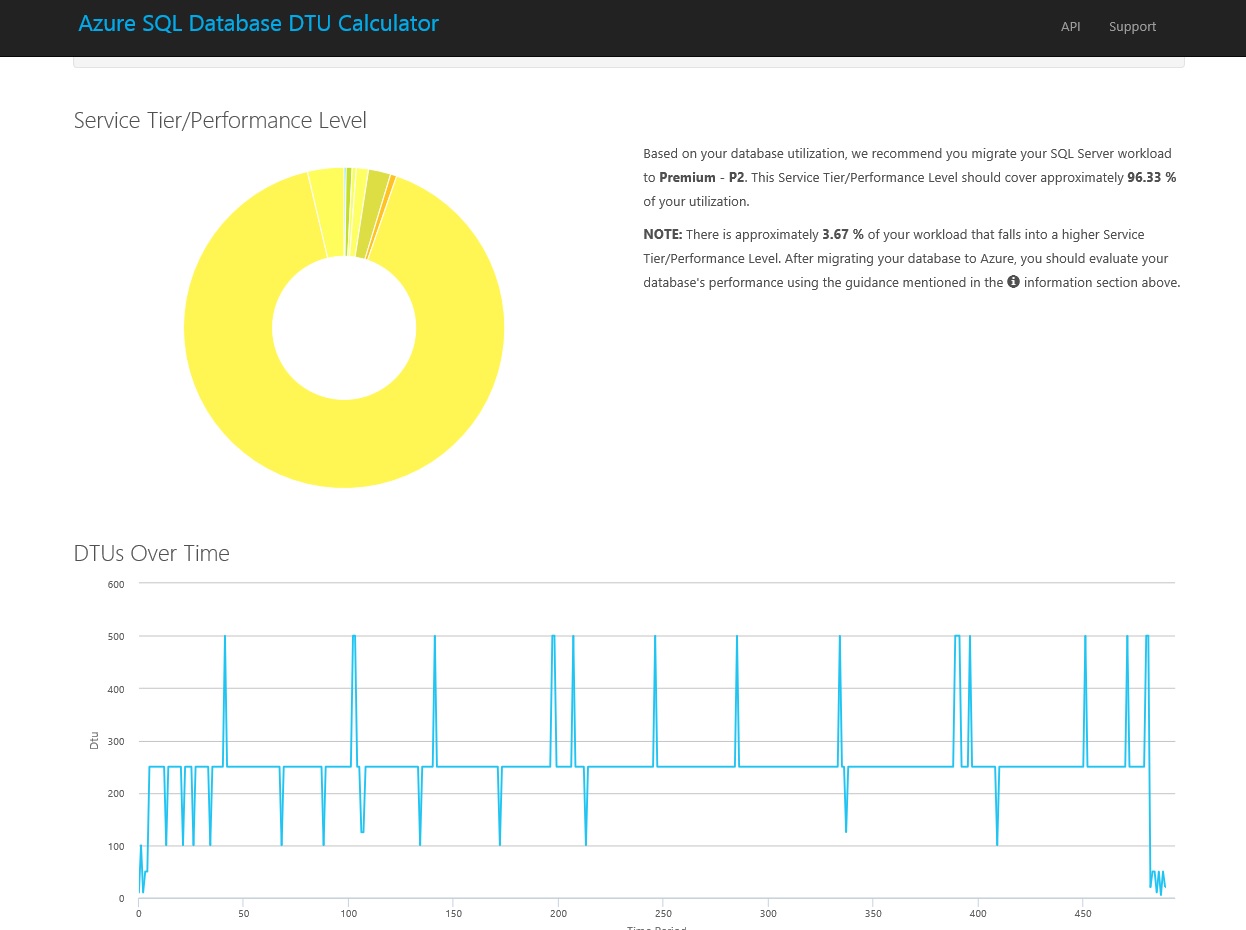
summary(subset(ca_OLAP$BatchDurationMS,ca_OLAP$AutomationEngine == "IO "& ca_OLAP$Description2 == "Two Concurrent Requests"))The ‘Azure SQL Database DTU Calculator’ service (see references) recommends a 'Performance Level’ for a given SQL Server workload. A representative workload is run on an existing server and performance counters are captured, these counters are then supplied to the DTU Calculator which makes a recommendation. A ‘DTU’ is a ‘Database Throughput Unit’, a suggestion of the CPU & IO resource requirements and service level, for a given workload on a given server. It’s calculated by capturing the performance counters below while the server is under load:
- Processor - % Processor Time
- Logical Disk - Disk Reads/sec
- Logical Disk - Disk Writes/sec
- Database - Log Bytes Flushed/sec
The CA benchmarking process (see references) was run on a local Hyper-V virtual server with Windows Server 2016 and SQL Server 2016, with 2 vCPU's and 8 GB of RAM. The performance counters were captured during the benchmark and passed to the DTU Calculator which suggested Premium - P2.
The same CA benchmark workload was then run on the VM & Azure (P2) using the parameters below, the results from both were saved as a single csv file and imported into R Studio.
| Concurrent Requests | @Batches | @IO_Benchmark | @CPU_Benchmark | @NewPatternsInBatch | @StressLevel | @Description1 |
| 2 | 10 | 1 | 0 | 50 | 2 | VM |
| 2 | 10 | 0 | 1 | 50 | 2 | VM |
| 2 | 10 | 1 | 0 | 50 | 2 | Azure |
| 2 | 10 | 0 | 1 | 50 | 2 | Azure |
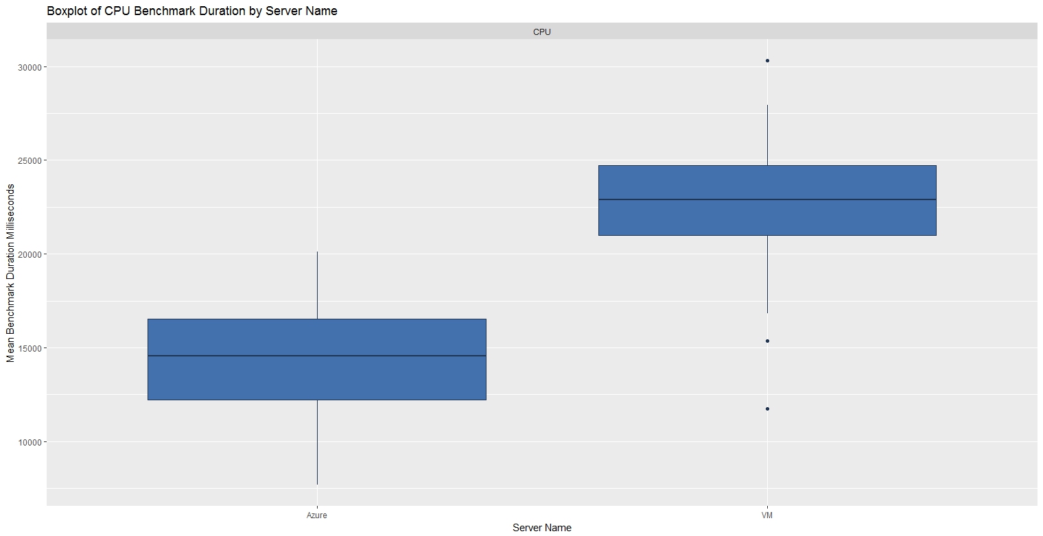
CPU Benchmark
SQL Azure CPU performance, at the recommended P2 level, was close to twice as fast as the VM.
| Benchmark | Min. | 1st Qu | Median | Mean | 3rd Qu | Max |
| CPU - VM | 11,733 | 21,004 | 22,890 | 22,581 | 24,703 | 30,307 |
| CPU - SQL Azure | 7,673 | 12,214 | 14,570 | 14,317 | 16,514 | 20,126 |
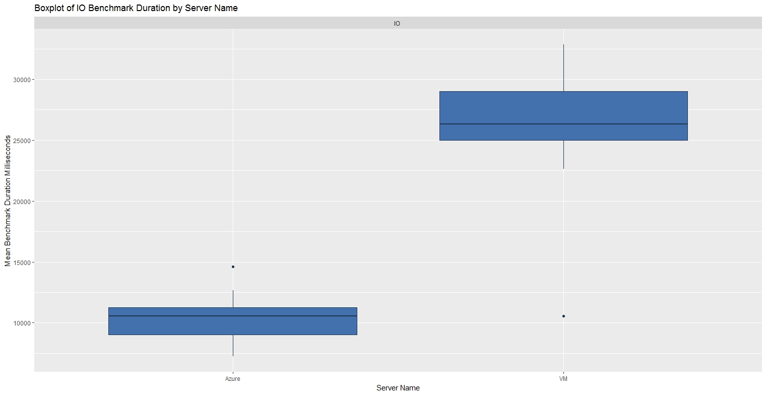
IO Benchmark
SQL Azure IO performance, at the recommended P2 level, was more than twice as fast as the VM.
| Benchmark | Min. | 1st Qu | Median | Mean | 3rd Qu | Max |
| IO - VM | 10,546 | 25,009 | 26,315 | 26,290 | 28,998 | 32,850 |
| IO - SQL Azure | 7,234 | 9,044 | 10,562 | 10,299 | 11,254 | 14,610 |
The T-SQL script below was then run in two concurrent query analyser sessions to produce the CA Benchmark workload, first on the VM then SQLAzure.
EXECUTE dbo.CA_Benchmark @Batches = 10 ,@CPU_Benchmark = 1 ,@IO_Benchmark = 1 ,@NewPatternsInBatch = 50 ,@DisplayPatterns = 0 ,@Initialize = 1 ,@StressLevel = 2 ,@Description1 = 'xx'
The results from the CA benchmarks in Azure and the VM were combined and saved as a csv file then imported into R and graphed using the script below:
rm(list=ls())
ca <- read.csv(file = "c:/DataScience/CA_Azure_20170930.csv", header = TRUE, sep = ",", stringsAsFactors = FALSE)

# Factors
ca$StartTime <- as.factor(ca$StartTime)
ca$BenchmarkPerspective <- as.factor(ca$BenchmarkPerspective)
ca$ServerName <- as.factor(ca$Description1)

#install.packages("ggplot2")
library("ggplot2")

ca_CPU <- subset(ca,ca$BenchmarkPerspective == "CPU")
ca_IO <- subset(ca,ca$BenchmarkPerspective == "IO ")

fill <- "#4271AE"
line <- "#1F3552"

# CPU Benchmark
p1 <- ggplot(ca_CPU, aes(x = ServerName, y = BatchDurationMS)) + geom_boxplot()
p1 <- p1 + scale_x_discrete(name = "Server Name") +
  scale_y_continuous(name = "Mean Benchmark Duration Milliseconds") +
  geom_boxplot(fill = fill, colour = line)
p1 <- p1 +  ggtitle("Boxplot of CPU Benchmark Duration by Server Name")
p1 <- p1 + facet_wrap(~ BenchmarkPerspective)
p1

# IO Benchmark
p2 <- ggplot(ca_IO, aes(x = ServerName, y = BatchDurationMS)) + geom_boxplot()
p2 <- p2 + scale_x_discrete(name = "Server Name") +
  scale_y_continuous(name = "Mean Benchmark Duration Milliseconds") +
  geom_boxplot(fill = fill, colour = line)
p2 <- p2 +  ggtitle("Boxplot of IO Benchmark Duration by Server Name")
p2 <- p2 + facet_wrap(~ BenchmarkPerspective)
p2

summary(subset(ca_CPU$BatchDurationMS,ca_CPU$ServerName == "VM"))
summary(subset(ca_CPU$BatchDurationMS,ca_CPU$ServerName == "Azure"))
summary(subset(ca_IO$BatchDurationMS,ca_IO$ServerName == "VM"))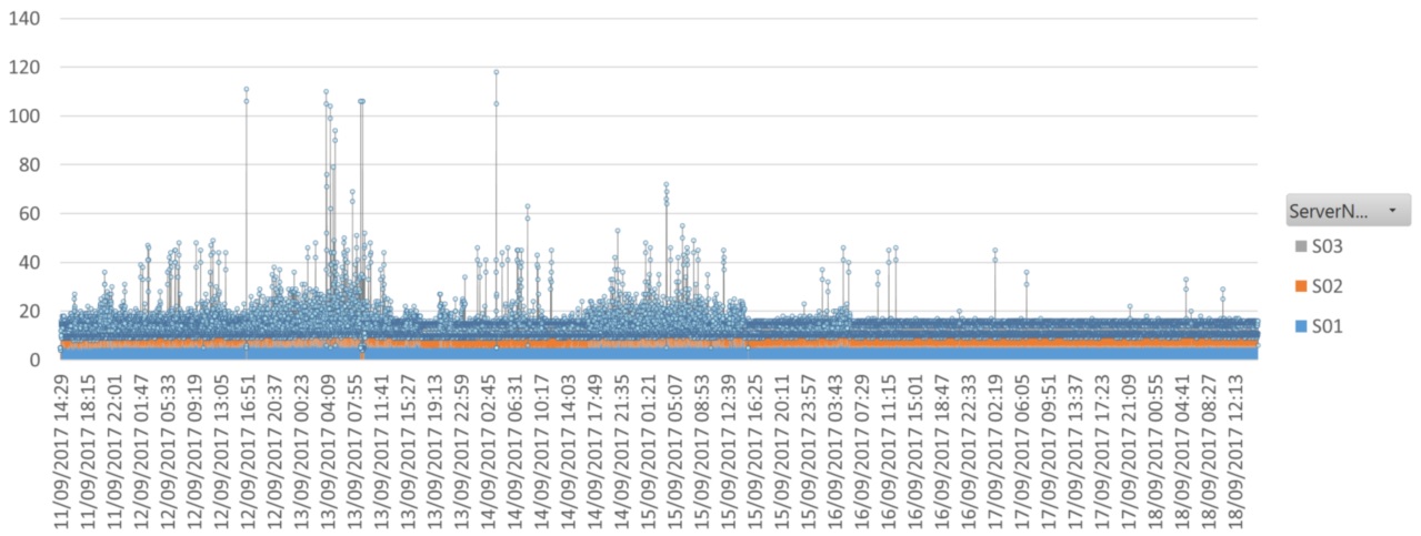
summary(subset(ca_IO$BatchDurationMS,ca_IO$ServerName == "Azure"))The CA Benchmark procedure can executed without parameters to take a small benchmark or 'Synthetic Transaction'. The graph below shows a busy development server hosting three instances of SQL Server 2012 under constant and consistent load. On the afternoon of the 15th September, a change was made and the available CPU count went from 20 to 60 for all three (non-affinitized) instances. The effect of the extra CPU's was evident in the improved consistency of the CA Benchmark times.
Suggested Usage
- Schedule a SQL Agent job to run 24 hours before any event likely to impact a SQL Server instance, take a default CA Benchmark (~5 seconds) at five minute intervals, disable the job 24 hours after the change. A comparison of the before/after results should show whether the change had any impact on the performance of client requests to the instance.
- After installing new SQL Server instances, take a predefined (SLA) CA Benchmark that places a representative load. This result in isolation isn't very interesting but subsequently, any other new SQL Server installations can have the same CA Benchmark taken and the relative performance of the servers can then be compared.
References
- http://en.wikipedia.org/wiki/Conway's_Game_of_Life - This Wikipedia link explains all the principles and patterns used in this article.
- https://www.mssqltips.com/sqlservertip/4210/extracting-showplan-xml-from-sql-server-extended-events/ - Extended Event session measured for observer overhead
- http://www.statmethods.net/management/subset.html
- The Hekaton Cellular Automation database setup script, ran before executing the scripts below.
- https://www.simple-talk.com/sql/database-administration/hekaton-in-1000-words/
- https://msdn.microsoft.com/en-gb/library/dn170449.aspx
- SQL Azure DTU Calculator - http://dtucalculator.azurewebsites.net/
- SQL Azure Performance – https://cbailiss.wordpress.com/2015/01/31/azure-sql-database-v12-ga-performance-inc-cpu-benchmaring/
License
SQL Server Cellular Automation Benchmarking is licensed under the MIT license, a popular and widely used open source license.
Copyright (c) 2017 Paul Brewer
The above copyright notice and this permission notice shall be included in all copies or substantial portions of the Software.
THE SOFTWARE IS PROVIDED “AS IS”, WITHOUT WARRANTY OF ANY KIND, EXPRESS OR IMPLIED, INCLUDING BUT NOT LIMITED TO THE WARRANTIES OF MERCHANTABILITY, FITNESS FOR A PARTICULAR PURPOSE AND NONINFRINGEMENT. IN NO EVENT SHALL THE AUTHORS OR COPYRIGHT HOLDERS BE LIABLE FOR ANY CLAIM, DAMAGES OR OTHER LIABILITY, WHETHER IN AN ACTION OF CONTRACT, TORT OR OTHERWISE, ARISING FROM, OUT OF OR IN CONNECTION WITH THE SOFTWARE OR THE USE OR OTHER DEALINGS IN THE SOFTWARE.
Appendix
The PowerShell script below was used to perform the benchmark tests in this article, OSTRESS is part of the RML tools for SQL Server (http://www.microsoft.com/en-gb/download/details.aspx?id=4511). Each line in the script was highlighted and run individually as running in a single batch caused unpredictable results:
cd "C:\Program Files\Microsoft Corporation\RMLUtils"
Set-Location .
cls

########################
# Hekaton / SQL
# Two concurrent requests
# OLTP
./ostress -SVM01 -dCA_SQLHekaton -n2 -r1 -Q"EXECUTE [dbo].[CA_Benchmark] @IO_Benchmark = 1, @Batches = 1000, @NewPatternsInBatch = 1, @StressLevel = 1, @Description1 = 'OLTP', @Description2 = 'Two Concurrent Requests', @Initialize = 1;" -o"C:\temp\log1"
./ostress -SVM01 -dCA_SQLHekaton -n2 -r1 -Q"EXECUTE [dbo].[CA_Benchmark] @Hek_Benchmark = 1, @Batches = 1000, @NewPatternsInBatch = 1, @StressLevel = 1, @Description1 = 'OLTP', @Description2 = 'Two Concurrent Requests', @Initialize = 1;" -o"C:\temp\log2"
# OLAP
./ostress -SVM01 -dCA_SQLHekaton -n2 -r1 -Q"EXECUTE [dbo].[CA_Benchmark] @IO_Benchmark = 1,@Batches = 10, @NewPatternsInBatch = 100, @StressLevel = 3, @Description1 = 'OLAP', @Description2 = 'Two Concurrent Requests', @Initialize = 1;" -o"C:\temp\log3"
./ostress -SVM01 -dCA_SQLHekaton -n2 -r1 -Q"EXECUTE [dbo].[CA_Benchmark] @Hek_Benchmark = 1, @Batches = 10, @NewPatternsInBatch = 100, @StressLevel = 3, @Description1 = 'OLAP', @Description2 = 'Two Concurrent Requests', @Initialize = 1;" -o"C:\temp\log4"

########################
# Hekaton / SQL
# One concurrent request
# OLTP
./ostress -SVM01 -dCA_SQLHekaton -n1 -r1 -Q"EXECUTE [dbo].[CA_Benchmark] @IO_Benchmark = 1, @Batches = 1000, @NewPatternsInBatch = 1, @StressLevel = 1, @Description1 = 'OLTP', @Description2 = 'One Concurrent Request', @Initialize = 1;" -o"C:\temp\log1"
./ostress -SVM01 -dCA_SQLHekaton -n1 -r1 -Q"EXECUTE [dbo].[CA_Benchmark] @Hek_Benchmark = 1, @Batches = 1000, @NewPatternsInBatch = 1, @StressLevel = 1, @Description1 = 'OLTP', @Description2 = 'One Concurrent Request', @Initialize = 1;" -o"C:\temp\log2"
# OLAP
./ostress -SVM01 -dCA_SQLHekaton -n1 -r1 -Q"EXECUTE [dbo].[CA_Benchmark] @IO_Benchmark = 1,@Batches = 10, @NewPatternsInBatch = 100, @StressLevel = 3, @Description1 = 'OLAP', @Description2 = 'One Concurrent Request', @Initialize = 1;" -o"C:\temp\log3"
./ostress -SVM01 -dCA_SQLHekaton -n1 -r1 -Q"EXECUTE [dbo].[CA_Benchmark] @Hek_Benchmark = 1, @Batches = 10, @NewPatternsInBatch = 100, @StressLevel = 3, @Description1 = 'OLAP', @Description2 = 'One Concurrent Request', @Initialize = 1;" -o"C:\temp\log4"


########################
# SQL
# MAXDOP=0
./ostress -SVM01 -dCA_SQLAzure -n2 -r1 -Q"EXECUTE [dbo].[CA_Benchmark] @IO_Benchmark = 1, @Batches = 1000, @NewPatternsInBatch = 1, @StressLevel = 1, @Description1 = 'OLTP', @Description2 = 'MAXDOP=0', @Initialize = 1;" -o"C:\temp\log1"
./ostress -SVM01 -dCA_SQLAzure -n2 -r1 -Q"EXECUTE [dbo].[CA_Benchmark] @IO_Benchmark = 1, @Batches = 10, @NewPatternsInBatch = 100, @StressLevel = 3, @Description1 = 'OLAP', @Description2 = 'MAXDOP=0', @Initialize = 1;" -o"C:\temp\log1"
# MAXDOP=1
./ostress -SVM01 -dCA_SQLAzure -n2 -r1 -Q"EXECUTE [dbo].[CA_Benchmark] @IO_Benchmark = 1, @Batches = 1000, @NewPatternsInBatch = 1, @StressLevel = 1, @Description1 = 'OLTP', @Description2 = 'MAXDOP=1', @Initialize = 1;" -o"C:\temp\log1"
./ostress -SVM01 -dCA_SQLAzure -n2 -r1 -Q"EXECUTE [dbo].[CA_Benchmark] @IO_Benchmark = 1, @Batches = 10, @NewPatternsInBatch = 100, @StressLevel = 3, @Description1 = 'OLAP', @Description2 = 'MAXDOP=1', @Initialize = 1;" -o"C:\temp\log1"

########################
# SQL
# XE OFF
./ostress -SVM01 -dCA_SQLAzure -n2 -r1 -Q"EXECUTE [dbo].[CA_Benchmark] @IO_Benchmark = 1, @Batches = 1000, @NewPatternsInBatch = 1, @StressLevel = 1, @Description1 = 'OLTP', @Description2 = 'XE OFF', @Initialize = 1;" -o"C:\temp\log1"
./ostress -SVM01 -dCA_SQLAzure -n2 -r1 -Q"EXECUTE [dbo].[CA_Benchmark] @IO_Benchmark = 1, @Batches = 10, @NewPatternsInBatch = 100, @StressLevel = 3, @Description1 = 'OLAP', @Description2 = 'XE OFF', @Initialize = 1;" -o"C:\temp\log1"

# XE ON
./ostress -SVM01 -dCA_SQLAzure -n2 -r1 -Q"EXECUTE [dbo].[CA_Benchmark] @IO_Benchmark = 1, @Batches = 1000, @NewPatternsInBatch = 1, @StressLevel = 1, @Description1 = 'OLTP', @Description2 = 'XE ON', @Initialize = 1;" -o"C:\temp\log1"
./ostress -SVM01 -dCA_SQLAzure -n2 -r1 -Q"EXECUTE [dbo].[CA_Benchmark] @IO_Benchmark = 1, @Batches = 10, @NewPatternsInBatch = 100, @StressLevel = 3, @Description1 = 'OLAP', @Description2 = 'XE ON', @Initialize = 1;" -o"C:\temp\log1"
SELECT CONVERT(VARCHAR(16),[BatchStartTime],120) AS StartTime
      ,[BatchDurationMS]
      ,[BenchmarkPerspective]
      ,Description1
      ,Description2
      ,Description3
FROM [dbo].[CA_BenchmarkResults]