Summary

This article aims at demystifying what grid search is and how we can use to obtain optimal values of our model parameters. It would be highly beneficial for the reader if the prequels to this article are read to gain a holistic understanding of the various techniques that can be used in optimizing the performance of our machine learning models.

The prequels to this article are :

1. Dimensionality Reduction Techniques - PCA, Kernel-PCA and LDA Using Python
2. Model Selection and Performance Boosting with k-Fold Cross Validation and XGBoost

Grid Search Intuition

For any Data Science problem we can divide the analytical aspects of the problem into six parts:

1. The first part would be the Data Preprocessing, which involves importing the dataset into our favorite IDE (Integrated Development Environment). In our case we would be using the Jupyter Lab of Anaconda Distribution as our Python IDE. This part includes cleaning the data, cleansing the data, and massaging the data. The latter involves taking care of missing values, taking care of categorical data (converting the string data into numerical data) and preparing the data for deeper structured analysis.
2. The second step would be to split the clean dataset into a Training Set and a Test Set. The training set is a subset of our data on which our machine learning model will learn how to predict the dependent variable with the independent variables. The test set is the complimentary subset from the training set, on which we will evaluate our model to see if it manages to predict correctly the dependent variable with the independent variables. We need to be cognizant of the fact that we do need to split our dataset on the dependent variable as well, as we want to have well distributed values of the dependent variable in the training and test set. For example, if we only had the same value of the dependent variable in the training set, our model wouldn’t be able to learn any correlation between the independent and dependent variables.
3. The third step would be to apply Feature Scaling to optimize the accuracy of our model predictions. Generally we should use normalization technique when the data is normally distributed, and scale (or use standardization) when the data is not normally distributed. When in doubt, we should go for standardization. However, what is commonly done is that the two scaling methods are tested. If feature scaling is not done, then a machine learning algorithm tends to weigh greater values, higher and consider smaller values as the lower values, regardless of the unit of the values and results would be biased(skewed).
4. The fourth step is to apply Feature Engineering dimensionality reduction techniques, like PCA, k-PCA and LDA (Feature Extraction), which has been discussed in detail in the prequel to this article. We can also use Feature Selection techniques like 'Backward Elimination' or a combination of both, which I will be discussing in my upcoming article.
5. The fifth step would revolve around the choosing of the actual machine learning model depending upon the problem we are trying to solve. There are many options available in like machine learning tool kit ranging from Regression techniques (both for linear and non linear problems) to Deep Learning techniques like ANN and CNN which I will be discussing in my upcoming articles.
6. The next steps would be to predict the test results and visualize the training and the test set results. We can then evaluate the effectiveness of our machine learning model using the techniques like Confusion Matrix and k-Fold Cross Validation which have been discussed in detail in previous articles (reduction techniques and model selection).
7. The last part is Hyperparameter tuning techniques like Grid Search and Random Search, in which we can try to further improve the performance and effectiveness of the prediction results of our machine learning model.

In this article we will be looking at one of the most widely used tool in the Data Scientists/AI Developer's tool kit which is the Grid Search. Grid search is a technique which helps to find the right set of hyperparameters for the particular model.

Difference between a parameter and a hyperparameter

Hyper parameters and parameters are very similar but not the exact same thing. A parameter is a configurable variable that is internal to a model whose value can be estimated from the data. A hyperparameter is a configurable value external to a model whose value cannot be determined by the data, and that we are trying to optimize (find the optimal value). An example might be the number of  'k-Folds' in the k-Fold Cross Validation technique, the number of trees  in ensemble methods like Random Forest through Parameter Tuning techniques like Random Search or Grid Search with k-Fold Cross Validation in combination.

Hyperparameters come through a lot of research and experimentation. There is no rule of thumb as to choose such numbers. Usually, we can find some ready to use neural networks architectures online which prove to get good results. But, we can experiment by tuning our model manually with other parameter values. And lastly, we can use the parameter tuning techniques like Grid Search with k-Fold Cross Validation to find the optimal values.

Implementation of Grid Search with k-Fold Cross Validation

To implement the k-Fold Cross Validation we will use the same sample 'Beer' dataset as demonstrated in the previous article before this article. First we import the necessary Python Modules into the IDE (Integrated Development Environment). Here we are using Jupyter Lab of Anaconda Distribution.

# Grid Search

# Importing the libraries
import numpy as np
import matplotlib.pyplot as plt
import pandas as pd

Next, we import the file named 'BeerDataset.csv' in the below step.

# Importing the dataset
dataset = pd.read_csv('BeerDataset.csv')

In the below code snippet, we read the columns from the 1st to the 12th of this 'BeerDataset' (the independent variables of this dataset) and assign it to 'X', which is a numpy array. Similarly we parse the result column of the dataset, which is the 'Beer_Grade' (the dependent variable), and assign it to 'Y', which is also a numpy array. Then we print the output and the type of variables 'X' and 'Y' as shown below.

# Assigning the Independent Variables to "X" and Dependent Variable Column to "y"
X = dataset.iloc[:, 0:13].values
y = dataset.iloc[:, 13].values

The next step would be divide the dataset into the training set and the test set. The training set is a subset of our data on which our model will learn how to predict the dependent variable with the independent variables. The test set is the complimentary subset from the training set, on which we will evaluate our model to see if it manages to predict correctly the dependent variable with the independent variables. To read more about the best practice in splitting the dataset into Training set and Test set read the previous article where in I have explained in detail about the steps of splitting the dataset.

The code snippet for dividing the dataset into Training and Test Set is as shown below:

# Splitting the dataset into the Training set and Test set
from sklearn.model_selection import train_test_split
X_train, X_test, y_train, y_test = train_test_split(X, y, test_size = 0.25, random_state = 0)

Next, we do feature scaling on the dataset. Feature Scaling techniques like normalization and standardization are used to normalize the range of independent variables or features of our dataset in order to avoid the results being skewed (biased) when dealing with multiple features spanning varying degrees of magnitude, range, and units. The steps from feature scaling till applying the dimensionality reduction technique of PCA is the same as illustrated in a previous article and can be found here.

I am also going to illustrate the same here as well so that we have the continuity of the flow for better understanding of the steps that need to be implemented and the Python code itself.

# Feature Scaling
from sklearn.preprocessing import StandardScaler
sc = StandardScaler()
X_train = sc.fit_transform(X_train)
X_test = sc.transform(X_test)

In this code snippet, we have imported the sklearn library to use the StandardScaler function. Set 'sc' to the StandardScaler() function. Further, we use fit_transform() along with the assigned object 'sc' to transform the data and standardize it. Standardization is only applicable on the data values that follow a Normal Distribution.

Next, we will use the Kernel-PCA dimensionality reduction technique the intuition and implementation steps of which have been explained in detail in the previous article. In the below code snippet, we import the KernelPCA() method from the sklearn.decomposition module. The kernel argument plays the same role as the covariance matrix in linear PCA, therefore we can calculate its eigenvalues and eigenvectors and stack them up to the selected number of components we want to keep.

# Applying Kernel_pca for getting a smother prediction boundary to capture all the real
# observation data points.

from sklearn.decomposition import KernelPCA
kpca = KernelPCA(n_components = 2, kernel = "rbf")
X_train = kpca.fit_transform(X_train)
X_test = kpca.transform(X_test)

We then apply the classifier technique kernel-SVM the intuition and implementation steps of which have been explained in the preceding article. Then the code snippet for the kernel-SVM would be as shown below:

# Fitting Kernel SVM to the Training set
from sklearn.svm import SVC
classifier = SVC(kernel = 'rbf', random_state = 0)
classifier.fit(X_train, y_train)

Right after the code computes the support vectors we have a 'Kernel - SVM'  classifier model fully trained on our training data, and ready to predict new predictions with the predict method, which is demonstrated in the below script.

# Predicting the Test set results
y_pred = classifier.predict(X_test)

We can calculate the confusion matrix and the code for confusion matrix is the same as we have seen in the previous article.

How much should we rely on the confusion matrix?

We can use the confusion matrix to get a sense of how potentially well our model can perform. However, we shouldn’t limit our evaluation of the performance to the accuracy on one train test split, as it is the case in the confusion matrix. First, there is the variance problem so we should rather apply k-Fold Cross Validation to get a more relevant measure of the accuracy.

The code to implement the k-Fold Cross Validation technique is as shown below:

# Applying k-Fold Cross Validation
from sklearn.model_selection import cross_val_score
accuracies = cross_val_score(estimator = classifier, X = X_train, y = y_train, cv = 10)

To understand the parameters of the cross_val_score method, which we imported from the sklearn.model_selection library. Refer to the predecessor article where in I have outlined in detail the step by step implementation and the best practices we need to consider.

We can then use the following metric depicted in the code snippet below to explain the evaluation of this classifier machine learning model 'Kernel - SVM'.

# Calculating the mean  and Standard Deviation of the 'Accuracy' Metric
accuracies.mean()
accuracies.std()

The mean accuracy resulting from all the 10 validation datasets is 95.5%.

Similarly the Standard Deviation  of the accuracies resulting from these 10 validation datasets is 4.8%.

This means the model can vary about 4.8%, which means that if we run our model on new data and get an accuracy of 95.5%, we know that this is like within 90.7 to 100% accuracy.

As mentioned earlier, we can now try to determine which is the best for model and the best parameters that will give us the best accuracy possible by implementing the Hyperparameter tuning techniques Grid Search, which is illustrated below. In the above code we used the kernel SVM to train our training set. Let us consider for understanding purposes, that we want to use the SVC model to train our training Set. Setting the optimal values of the hyper-parameters can be challenging and resource-demanding. We can imagine how many permutations we need to determine the best parameter values. This is where Grid Search Parameter tuning(estimation) technique of the machine learning tool-kit comes in handy.

# Applying Grid Search to find the best model and the best parameters
from sklearn.model_selection import GridSearchCV
parameters = [{'C': [1, 10, 100, 1000], 'kernel': ['linear']},
              {'C': [1, 10, 100, 1000], 'kernel': ['rbf'], 'gamma': [0.1, 0.2, 0.3, 0.4, 0.5,
               0.6,0.7, 0.8, 0.9]}]
grid_search = GridSearchCV(estimator = classifier,
                           param_grid = parameters,
                           scoring = 'accuracy',
                           cv = 10,
                           n_jobs = -1)
grid_search = grid_search.fit(X_train, y_train)
best_accuracy = grid_search.best_score_
best_parameters = grid_search.best_params_

If you have trouble importing the ’GridSearchCV’ on your local machine you can try to replace

from sklearn.model_selection import GridSearchCV

by:

from sklearn.cross_validation import GridSearchCV

although it depends on the system and package version also.

Grid search is a hyperparameter tuning technique that attempts to compute the optimum values of hyperparameters. It is an exhaustive search that is performed on a the specific parameter values of a model. The model is also known as an estimator. Grid Search can save us tremendous amount of time, effort and resources.

Hyper-parameters are parameters that are not directly learnt within estimators. In scikit-learn they are passed as arguments to the constructor of the estimator classes. Typical examples include C, kernel, gamma for Support Vector Classifier, aplha for Lasso, etc. The parameters of the estimator used to apply these methods are optimized by cross-validated grid-search over a parameter grid. It is possible and recommended to search the hyper-parameter space for the best cross validation score.

The 'C ' in the above code snippet is a penalty parameter is a regularization parameter that can allow us to do two things:

• reduce overfitting,
• override outliers.

It is equal to 1/? in where ? is the classic regularization parameter used in Ridge Regression, Lasso, Elastic Net.

A good start is to take default values and experiment with values around them. For instance, the default value of the penalty parameter C is 10, so some relevant values to try would be 1, 10 and 100. The grid search provided by GridSearchCV exhaustively generates candidates from a grid of parameter values specified with the param_grid parameter. For example, in the above code script of GridSearch 'parameters' specifies that two grids should be explored -  one with a linear kernel and C values in [1, 10, 100, 1000],  and the second one with an RBF kernel, and the cross-product of C values ranging in [1, 10, 100, 1000] and gamma values in [0.1, 0.2, 0.3, 0.4, 0.5, 0.6, 0.7, 0.8, 0.9].

# Printing out the grid search variable
grid_search

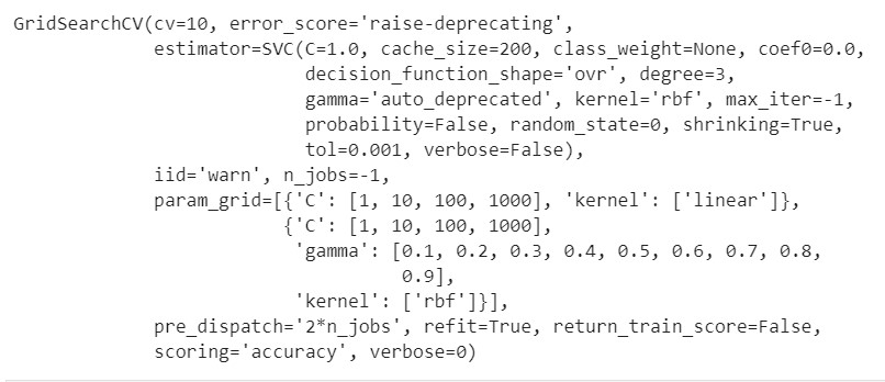
We can see from the above GridSearchCV output that GridSearchCV instance implements the usual estimator SVC which was the original machine learning model which we used to train our Training Set (kernel-SVM) and the param_grid uses the grid of parameter values specified in 'parameter' object.

The best accuracy that can be achieved by implementing the recommendation provided by the Grid Search technique (as shown in the below code snippets) is 96.9%.

#Printing the output of the 'best_accuracy' object
best_accuracy

The best parameters resulting by applying this Grid Search technique are:

#Printing the output of the 'best_parameters' object
best_parameters

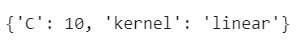
After implementing the Grid Search model the best parameters which will help us get a prediction accuracy of test set of 96.9% would be with a 'linear' kernel and a penalty parameter ,C=10. For more information see the API for RandomizedSearchCV and the Randomized Parameter Optimization section in the user guide.

If we then, as per the recommendation of GridSearch replace this code snippet from the above :

# Fitting Kernel SVM to the Training set
from sklearn.svm import SVC
classifier = SVC(kernel = 'rbf', random_state = 0)
classifier.fit(X_train, y_train)

with

# Fitting 'Linear'Kernel SVM to the Training set
from sklearn.svm import SVC
classifier = SVC(kernel = 'linear', random_state = 0)
classifier.fit(X_train, y_train)

and rerun the same code we get an accuracy of 96.9% when we used the SVM linear classifier versus the previously used kernel-SVM classifier. This gave a model accuracy of 95.5%.

Visualizing the results of the Training set using the below script, we get the following output.

# Visualising the Training set results
from matplotlib.colors import ListedColormap
X_set, y_set = X_train, y_train
X1, X2 = np.meshgrid(np.arange(start = X_set[:, 0].min() - 1, stop = X_set[:, 0].max() + 1, step = 0.01),
                     np.arange(start = X_set[:, 1].min() - 1, stop = X_set[:, 1].max() + 1, step = 0.01))
plt.contourf(X1, X2, classifier.predict(np.array([X1.ravel(), X2.ravel()]).T).reshape(X1.shape),
             alpha = 0.75, cmap = ListedColormap(('red', 'green', 'blue')))
plt.xlim(X1.min(), X1.max())
plt.ylim(X2.min(), X2.max())
for i, j in enumerate(np.unique(y_set)):
    plt.scatter(X_set[y_set == j, 0], X_set[y_set == j, 1],
                c = ListedColormap(('red', 'green', 'blue'))(i), label = j)
plt.title('SVM -> Linear - Kernel (Training set)')
plt.xlabel('PC1')
plt.ylabel('PC2')
plt.legend()
plt.show()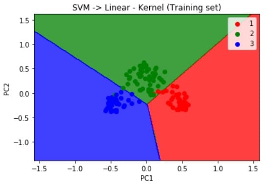

Similarly using the below code when we visualize the results of the Test set results we get the graph as illustrated below:

# Visualising the Test set results
from matplotlib.colors import ListedColormap
X_set, y_set = X_test, y_test
X1, X2 = np.meshgrid(np.arange(start = X_set[:, 0].min() - 1, stop = X_set[:, 0].max() + 1, step = 0.01),
                     np.arange(start = X_set[:, 1].min() - 1, stop = X_set[:, 1].max() + 1, step = 0.01))
plt.contourf(X1, X2, classifier.predict(np.array([X1.ravel(), X2.ravel()]).T).reshape(X1.shape),
             alpha = 0.75, cmap = ListedColormap(('red', 'green', 'blue')))
plt.xlim(X1.min(), X1.max())
plt.ylim(X2.min(), X2.max())
for i, j in enumerate(np.unique(y_set)):
    plt.scatter(X_set[y_set == j, 0], X_set[y_set == j, 1],
                c = ListedColormap(('red', 'green', 'blue'))(i), label = j)
plt.title('SVM -> Linear - Kernel (Test set)')
plt.xlabel('PC1')
plt.ylabel('PC2')
plt.legend()
plt.show()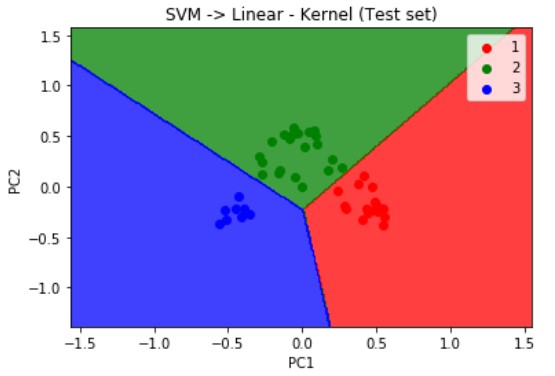

As mentioned earlier, when we used the linear SVM classifier to train our model,  we can deduce from the visualization results on the graph that the prediction boundary is a straight line.

Conclusion

In this article, we just saw how we can use the Grid Search to obtain optimal hyperparameters for a machine learning model that will enable us to have the best accuracy for the prediction of our east set results.

Next Steps

• Watch out for an upcoming article on step by step code on how to apply various Regression, Classification, Clustering, Association Rule Learning, Reinforcement Learning, NLP and Deep Learning techniques using Python where we will look at some of the most popular techniques and how to evaluate thier performance.
• How to implement automatic Backward Elimination in Python with and without Adjusted R-Squared ?
• For more examples on sample dataset pre-processing steps to prepare the data for more deeper structured analysis read my article on 'Comparing Two Geospatial Series with Python' and 'Reading a Specific File from an S3 bucket Using Python'.
• To gain a holistic overview of how Diagnostic, Descriptive, Predictive and Prescriptive Analytics can be done using Geospatial data, read my recent paper, which has been published on advanced data analytics use cases pertaining to that.