"Where two or three tables are related in my name, I am there among them" - Book of Microsoft 18:20
For beginners to Power Pivot or the Tabular Model, relating tables together can be one of the biggest stumbling blocks. What can make it especially challenging is that DAX relationships don't behave like SQL JOINs, which is what most of us are used to. Since DAX is not a query language like SQL, joining data requires a different approach. The following post is a crash course in relationships: how they work, when they work, and what you should do when they don't. The same techniques and fields are the same whether you're using Power Pivot or the Tabular Model.
The Basic Relationship
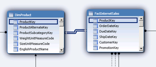
Relationships can be created and edited in two interfaces. The Diagram view (Model -> Model View -> Diagram View) denotes them with an arrow between tables:
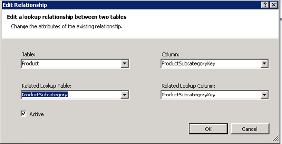
The Edit Relationships box (Table -> Manage Relationships) spells out, a bit more clearly, each table and column.
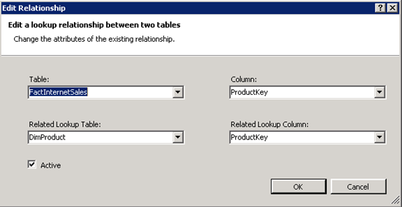
As you can see, relationships are not bidirectional. They require a "base" table and column, and a related lookup table and column. In the diagram view, the arrow points to the lookup table. It's vital to understand that different rules govern the two:
- The lookup column must have unique values.
- Every value in the base column must also be present in the lookup table. (That is, the base column can't have more unique values than the lookup column).
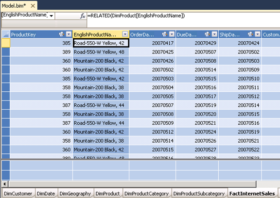
How do these rules play out? In the above example, you can go to FactInternetSales and add a calculated column for "EnglishProductName," which will be populated by referencing the ProductKey. The code is:
=RELATED(DimProduct[EnglishProductName])
You can see this in my worksheet below:
As you might surmise, relationships are built to reference dimension tables from fact tables, using a key. However, it's quite possible you'll want to do the opposite. For instance, let's say you want to see the total sales amount for each product, within the DimProduct table. You can still use the relationship, but you'll need a little more code:
=CALCULATE(Sum(FactInternetSales[SalesAmount]),USERELATIONSHIP(DimProduct[ProductKey],FactInternetSales[ProductKey]))
Here is the formula to show the sales.
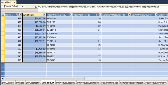
So how does this work? In FactInternetSales, the ProductKey isn't unique. The reason we can go "backwards" in our relationship, and use a non-unique key, is because we're aggregating SalesAmount BY ProductKey, and then relating with ProductKey.
More specifically: CALCULATE is behaving like GROUP BY in SQL. The first argument is an expression, which in this case is the sum. This gives us our actual value. The second argument is a filter. CALCULATE starts with the entire SalesAmount sum, within the FactInternetSales table. Then for each row of that table, it filters the sum by ProductKey. USERELATIONSHIP is necessary because our relationship depends on a calculation, instead of two existing columns that follow relationship convention.
So if you want to reference the base table from the lookup table, you'll need some kind of additional calculation. Don't try switching the base table and the lookup table--the direction of their relationship can't be changed, since the direction depends on which table has the unique keys.
Another nuance about PowerPivot relationships is the active/inactive relationship distinction. Each table can only tolerate a single active relationship in the same direction. Let's say the Product Subcategory table relates to the Product table, using the ProductSubcategoryKey:
If we try to establish another relationship between the tables, but using ProductSubcategory name instead, our new relationship is a dotted line, as shown below:
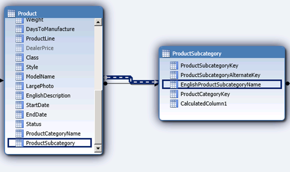
This signifies it as inactive. We could edit our first relationship, uncheck the "active" box, and use this one instead. But that's not necessary, since we can just use different syntax in our columns. (Admittedly, this example is a bit redundant, since the SubcategoryName field can already be referenced with our first relationship…but it at least demonstrates the point).
To use an inactive relationship, you use the, guess what, USERELATIONSHIP function!
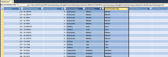
=CALCULATE(VALUES(ProductSubcategory[EnglishProductSubcategoryName]),USERELATIONSHIP(ProductSubcategory[EnglishProductSubcategoryName],Product[ProductSubcategory]))
Again, CALCULATE encapsulates the whole function. Its 1st argument, expression, is the field we want to reference in the other table. However, we have to use VALUES around it. VALUES makes certain that the referenced field returns single rows, and not any kind of aggregation. It's often used with CALCULATE functions that should return a dimensional value. The USERELATIONSHIP function is the filter argument of CALCULATE establishes the 1st column to use as the lookup, and the 2nd to use as the base. (Again, ProductSubcategory is the lookup, since it contains the unique lookup key).
However, in my experience, it's easier to avoid worrying about inactive and active relationships, and instead use functions that don't require relationships at all.
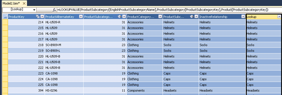
The first is LOOKUPVALUE, which is a simpler version of VLOOKUP in Excel. Its argument takes a result column (from the lookup table), a search column (from the lookup table) and a search value (from the base table, which matches with the search column). The result…is the result column!
So my function reads:
=LOOKUPVALUE(ProductSubcategory[EnglishProductSubcategoryName],ProductSubcategory[ProductSubcategoryKey],Product[ProductSubcategoryKey])
Your other option is using CALCULATE in conjunction with FILTER. This is especially helpful if your lookup table doesn't have unique keys--perhaps it's a fact table. In these cases, and potentially many others, you'll want to reference an aggregate in the lookup. LOOKUPVALUE won't work, since its arguments doesn't allow further filtering. So if I wanted to reference the FactInternetSales table, and lookup the most recent purchase for each product, all within the Product table, I would use this:
=CALCULATE(MAX(FactInternetSales[OrderDateKey]),FILTER(FactInternetSales,FactInternetSales[ProductKey]=Product[ProductKey]))
The first argument of CALCULATE is a MAX aggregation, which provides us with a single value to use as the lookup key. The second argument is simply a filter, which takes as its argument the target table, and then the filter condition. The filter condition, which is just LookupColumn = BaseColumn, relates the tables much easier than an actual relationship.
However, one of the advantages of using actual relationships is their inheritance. For instance, the ProductCategory table is related to the ProductSubcategory table.
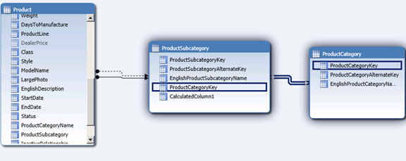
We can reference ProductCategory from Product, even though they're not directly related:
=RELATED(ProductCategory[EnglishProductCategoryName])
Here, a base table is referencing its lookup table, which then performs its own lookup. If you have several layers of dimensional tables, this can be a real time-saver.
About the Author
Michael Carper is a business intelligence consultant at Apparatus.