Introduction

In response to my approach in the popular MDX Guide for SQL Folks series. I am using SQL as a good frame of reference for starting or developing a new approach for improving your Data Analysis Expression(DAX) language learning experience in this series. This is useful for developers starting to learn the DAX language to more advanced developers who have struggled to adjust to the language coming from a SQL background.

In Part I of the series, we discussed some very important Data Visualization and Tabular Model concepts that are essential to the DAX learning process esp. when coming from a SQL background,

In Part II we continued the DAX language learning process by translating SQL queries to DAX Queries, all the time emphasizing the functional nature of DAX.  We looked at DAX Queries using the EVALUATE and SUMMARIZCOLUMS keywords as they would be used in SSMS and DAX Studio and other client query tool similar to writing SELECT statements in SQL.

In Part III, we are going to look at how to use DAX formulas to create calculations one can use in Power BI reports. We will first look at the two types of calculations you can create in a Tabular Model using Power BI, namely, Calculated Column and Calculated Measures. We will outline the major differences between the two types of calculations, and finally, we will have an introductory look at a few key DAX function groups very useful and often used in DAX formulas.  For the rest of the series, all the examples will be demonstrated with and within Power BI Desktop.

Part III - DAX Calculations

In Part II, we were exposed to some DAX calculations through Query Measure. These were predefined calculations you could use in your query. In this part, we are going to talk about predefined calculations (similar to Query Measure ) that you can use as values and fields in Power BI report.

Transitioning from DAX Queries to DAX Calculation

In part II we learned about DAX queries with a typical summary functional syntax as below ;

     Summary Functional Syntax:

EVALUATE((SUMMARIZECOLUMNS(FILTER(),SUM())))

In DAX queries, the required and often the outer-most function is EVALUATE, because EVALUATE is DAX's equivalent of the SQL SELECT clause.

In DAX Calculations in Power BI, we don’t use the EVALUATE function because Power BI applies that to the formula for us. Secondly, in a calculation, we will mostly aggregate data and use operators rather than project multiple columns, therefore, we will not use SUMMARIZECOLUMNS which is a column projection function. In effect, most of the typical outer functions you will use in these formulas are going to be aggregation functions that aggregate various expressions involving the use of your typical calculation operators like +, -, / etc.

Thus the core of most DAX Calculation functional syntaxes will usually of the forms below;

Summary Functional Syntaxes:

  SUM(FILTER(..))
  SUMX(FILTER(..))
  CALCULATE(SUMX(FILTER(..)))

We will learn how these functions work, but here again, the complexity of the code will be determined by the complexity of the expressions that one uses as arguments for these aggregation and filtering outer function. Apart from the functional syntax changes noted here, everything you learned in Part I and Part II about DAX still applies, i.e. Relationships, Expanded Tables and Functional language syntax, etc.

Power BI Desktop

Download and install Power BI, and connect to the tabular model database we installed in Part II. For those completely new to Power BI, I will recommend this how-to tutorial Get started with Power BI Desktop. It shows you how to install Power BI, connect to data sources, and also create Calculation and use them Power BI reports.

DAX Calculations in Power BI

DAX calculations are created using formulas. We will be entering all formulas in Power BI in the rest of the series. All formulas will have elements as shown in figure 1 below.

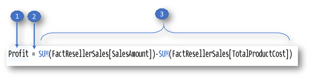
                                                       figure 1; Showing the various elements of a DAX formula

The formula syntax element labeled in figure1 are explained below:

1. The name of the Calculation or Expression.
2.  Equals sign (=) which is an operator indicating the start of the DAX formula and equating the two sides.
3. DAX Calculation or Expression formula syntax.

There are two primary calculations or expressions you can create in Power BI or Tabular Model using DAX namely Calculated Columns and Calculated Measures.

Calculated Columns allow you to extend a table by creating new columns. The content of the columns is defined by a DAX expression evaluated row by row. They are useful when you want to slice or filter on the value, or if you want a calculation for every row in your table.

Calculated Measures presents another way of defining calculations in a DAX model, useful whenever you do not want to compute values for each row but, rather, you want to aggregate values from many rows in a table. A Calculated Measure creates a field having aggregated values such a sum, ratios, percentages, averages, etc.

In Part II we explored Query Measures which are calculation defined within the scope of a query. Essentially, Calculated Measure lets you create the same calculations but unlike Query Measures, Calculated Measures are persisted in the model making them global and available for use in reports by anyone with access to the model. Normally you test complex calculations in a query using Query Measures and then move it into the model as  Calculated Measures so that they can be used in a report.

Creating DAX Calculations

In this section, we will learn how to create some simple calculations and reports using Power BI.  For those completely new to these topics, you can check out these tutorials.

Creating Calculated Columns

In Power BI Desktop we will create a new Calculated Columns called Profit1 in the factResellerSales Table. To do this follow the 5 steps outlined in the figures below.

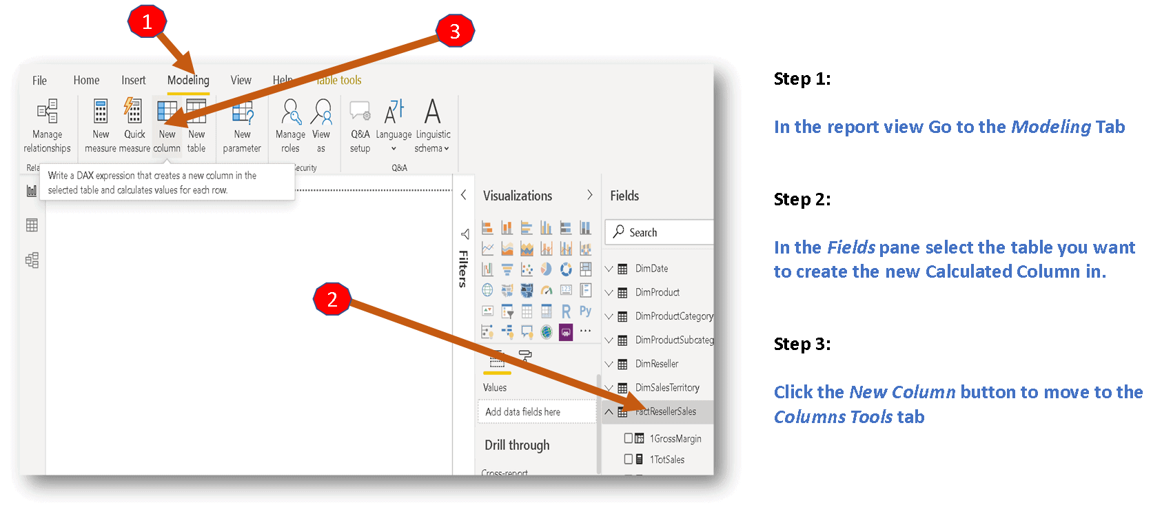
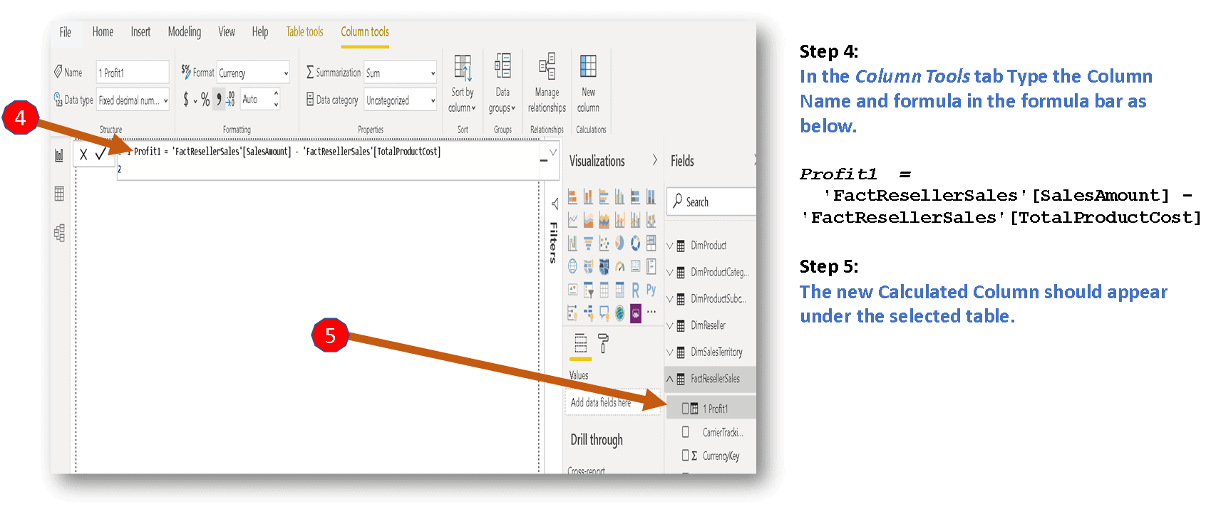
              Figure 2: Showing the steps to create a Calculated Column

The required elements for a calculated column are the following:

• a new column name
• at least one function or expression

If you reference a table or column in your calculated column formula, you do not need to specify a row in the table - Power BI calculates the column for the current row for each calculation.

Creating Calculated Measures

We will also create a new Calculated Measure called Profit2 in the factResellerSales Table. To do this follow the 5 steps outlined in the figures below.

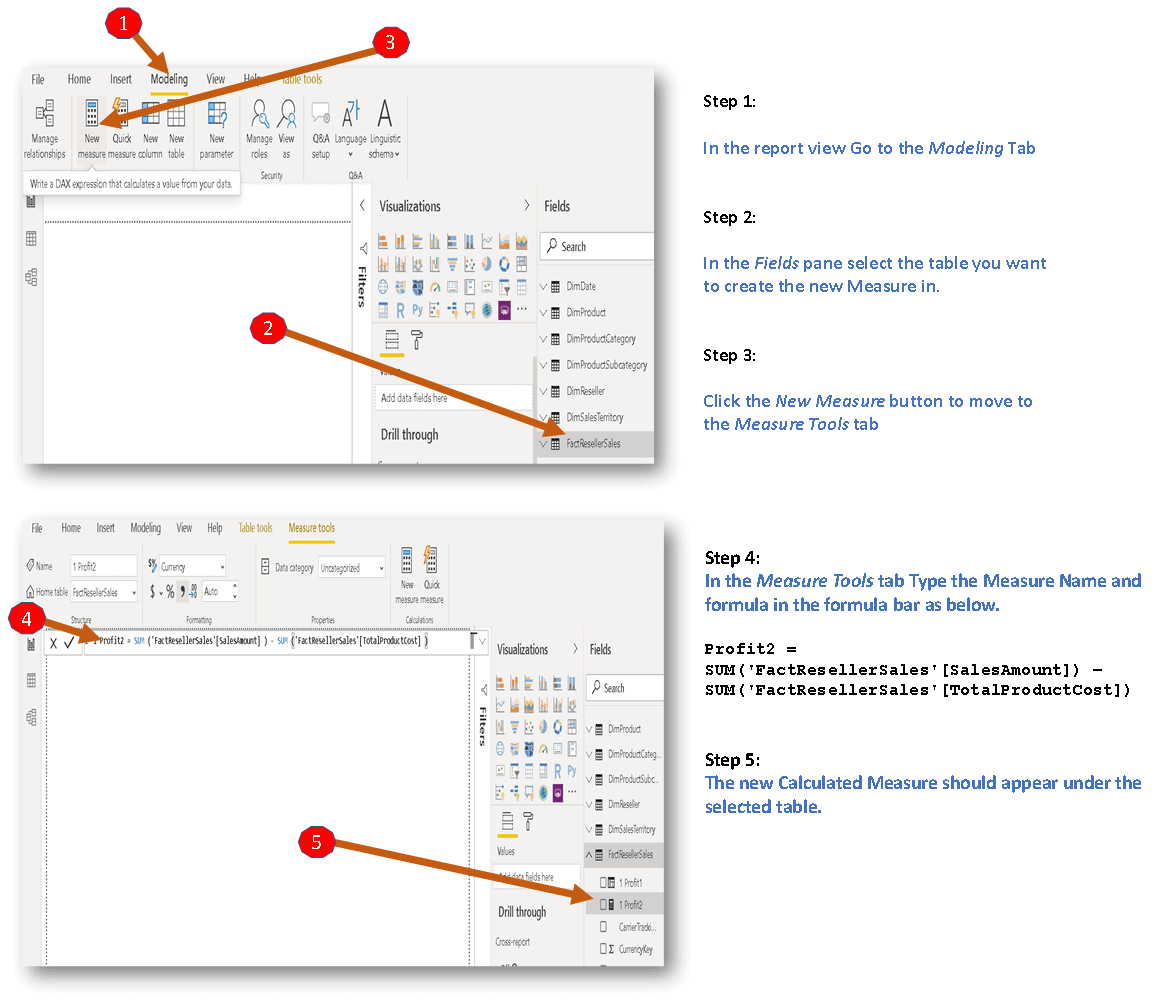
    Figure 3: Showing the steps to create a Calculated Measure

The required elements for a calculated measure are the same as they are for a calculated column: Once you create the measure, you can modify your measure name with a calculator icon next to it, under the table name you created the measure in.

Syntax & Convention

In creating the two calculation types above the equals sign (=) operator was used both as shown in step 4 in each case. In the remainder of the series, we will differentiate  Calculated Columns from Calculated Measure by adopting the operator sign below.

  =                 Calculated Column reference

 :=                 Calculated Measure reference

So the two formulas we entered above in steps 4 will be represented as in Listing 1 and Listing 2 below.

Listing 1 (Calculated Column):

'FactResellerSales'[Profit1] = 'FactResellerSales'[SalesAmount] - 'FactResellerSales'[TotalProductCost]

Listing 2 (Calculated Measure):

'FactResellerSales'[Profit2]:= 
SUM ('FactResellerSales'[SalesAmount] ) – SUM ('FactResellerSales'[TotalProductCost] )

Note that the table name 'FactResellerSales' is added to the name of the formula in the Listings to indicate the table hosting the calculation.

Using Calculations in Power BI Report

Creating reports with calculations and other columns in Power BI is easy. Figure 4 below is a simple Power BI report with a table and a chart built using the profit calculations we created above.

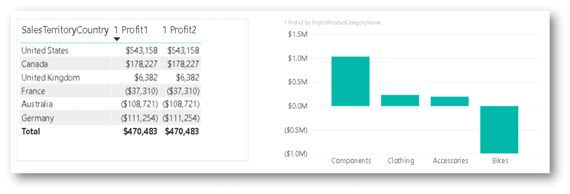
                                        Figure 4: Showing a table and a chart on a report using profit calculations.

The steps in figure 5 below showing how to create the table in the report.

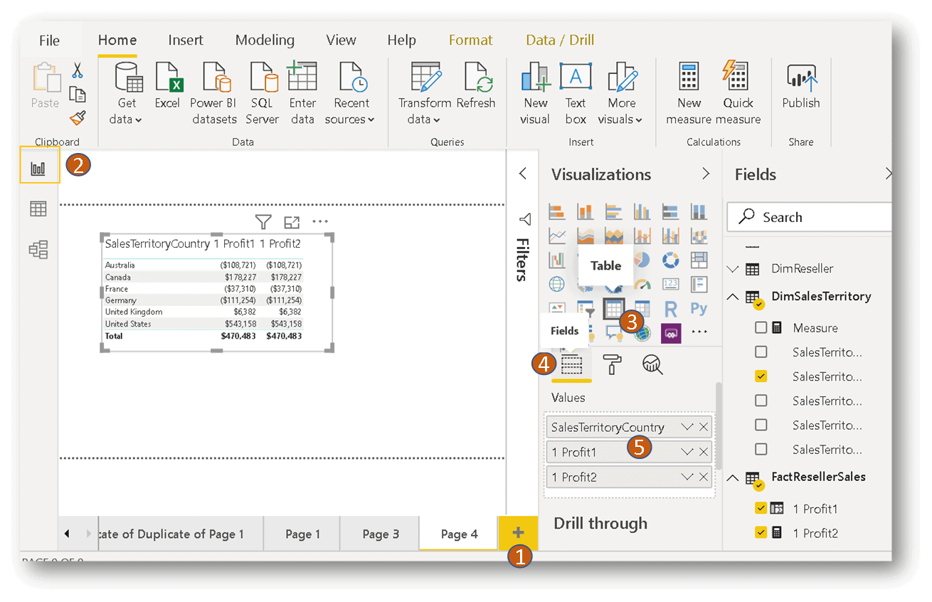
           Figure 5: Showing how to create a table in a Power BI report.

Steps:

1. Click the + sign on the pages tab area at the bottom of the screen to create a new report page.
2. Click on the charts ribbon to make sure you are in the default Reports Mode.
3. Under Visualizations pane click to select the Table visual to display a table visual on the canvas in the report page.
4. Click on the Fields ribbon under Visualizations to highlight the Values sections.
5. Drag and drop the  SaleTerritoryCountry columns from DimSalesTerritory table under the Fields Pane unto the Values section. Do the same by dragging and dropping the Profit calculations from the FactResellerSales table.

Try and follow the same steps to create the Chart on the report. For those completely new to Power BI reports check out the Build reports section of the Get started with Power BI Desktop how-to tutorial to learn more about creating reports.

Choosing between Calculation Types

More often than not both Calculation types can produce the result. Therefore to understand when and how to use each one must understand their pros and cons. Below are some key points one has to consider when choosing between Calculated columns and Calculated Measures.

    Calculated Columns

• Calculated columns are columns in a table that are computed with a DAX expression. They are computed once during table processing and are computed again at data refresh time.
• Because the column is calculated, the result is consolidated in the table and does not change according to the user selection in the report
• They are stored in the database, just like any other column
• Tabular storage is in-memory, therefore all calculated columns occupy space in memory
• Because the time required to compute them is always process time and not query time, they result in better user experience when used in Reports. The downside is that you must always remember that a calculated column uses precious RAM.

  Calculated Measures

• Unlike Calculated Columns that are computed at data refresh, Calculated Measures are computed at query time. Consequently;
  • the value of a Calculated Measure depends on the user selection in the report.
  • demanding measure calculations may not result in better user experience compared to calculated columns.
• Unlike Calculated Columns, the computations are not stored in the tables and thus do not end up consuming precious RAM.

Choosing between the two types of calculations becomes more crucial with large datasets. When the size of the model is not an issue, you can use the method you are more comfortable with. However, as a rule, one should limit the use of calculated columns to the few cases where they are strictly needed. In other words, whenever you can express a calculation both ways, choose Calculated Measures over Calculated Columns.

For more on how to choose between calculated columns and measures, you can check out this article Calculated Columns and Measures in DAX by Marco Russo

Introduction to Aggregators and Iterators

A major aspect of Analytics is about aggregating data and Tabular Model and DAX offers developer various opportunities to do that. DAX offers two functional groups that aggregate data in DAX calculations, namely, Aggregators and Iterators. We are going to look at the two types and how they are used.

Aggregators

DAX Aggregators are similar to aggregate functions available in SQL and their use is also similar. In DAX, these comprise of functions from the Math and Statistical function groups including functions like SUM, COUNT, AVERAGE, MIN, MAX, STDEV, RANK, etc. Like in SQL they perform aggregation on data.  They aggregate the values of a column in a table and return a single value with a general syntax as below.

     AggFunction(<column>)

• Column;  The column that contains the values to be Aggregated.

The most familiar is probably the SUM function. In the example below the function is used in a Calculated Measure to sum of all the numbers in the SalesAmount column of the FactResellerSales table:

Listing 3:

 'FactResellerSales'[Sales] := SUM('FactResellerSales'[SalesAmount] )

• When used in Calculated Columns aggregators are similar to their SQL counterparts; SUM aggregates all the rows of the table column.
• On the other hand, when they are used in a Calculated Measure, they aggregate the rows that are being filtered by slicers, rows, columns, and filter conditions in the report (We will look at the effects of these "external" filters in next parts of the series).

All the aggregation functions work on columns therefore, they aggregate values from a single column only. For instance, if you try to run the formula in listing 4 below you will receive the error message below

Listing 4:

WrongProfit:=
     sum('FactResellerSales'[SalesAmount] - 'FactResellerSales'[TotalProductCost])

Error: The SUM function only accepts a column reference as an argument

Note that the behavior of the other the aggregators  (AVERAGE, MIN, MAX, and STDEV) are similar to that of SUM as explained above, the difference is only in the way they aggregate values. Apart from MIN and MAX that can operate on text values, they all operate only on numeric values or dates.

Iterators

Iterators are some of the most important functions you will use in DAX. Unlike the aggregators we encountered above, Iterators are aggregation functions that can aggregate an expression instead of a single column. Iterators accept at least two arguments with general syntax as below;

AggFunctionX (<Table>, <Expression>)

• They are referred to as Iterators because they operate on data row by row.
• The Table argument represents a table or an expression that returns a table that they scan.
• The Expression argument is an expression that is evaluated for each row of the table.

Firstly, Iterators scan the table or records provided as the first argument. Secondly, they evaluate the expression provided as the second argument row by row. Finally,  they aggregate the partial results according to the particular aggregator semantics.

Most iterator functions are suffixed with X and have the same name as their noniterative counterpart. For example, SUM has a corresponding SUMX, and MIN has a corresponding MINX, etc, as below.

SUMX, COUNTX, AVERAGEX, MINX, MAXX, STDEVX, RANKX

Notes: Firstly, there are a few other functions like FILTER, GENERATE that are considered iterators even if they do not aggregate their results or have noniterative counterparts.  Secondly, even though most iterators accept two arguments as shown in the general syntax above,  a few iterators accept additional arguments after the first two. For example, RANKX is an iterator that accepts more than two arguments.

As can be seen from the general syntax of iterator above, the nature of the arguments provides a lot more opportunities to use them to perform aggregation on calculations based on complex expressions derived from a complex set of data compared to Aggregators. We will see how to utilize the arguments of these functions to create complex calculations in the following sections.

Simple iterations

Let's look at a simple iteration logic using the SUMX function. Let's say we want to create a Calculated Measures that will provide the freight charges to be used in reports. The result can be obtained with the SUMX function as shown in Listing 5 below.

Listing 5:

'FactResellerSales'[freightCharges] :=
SUMX(
             'FactResellerSales'
             ,'FactResellerSales'[Freight]
)

In the example above the SUMX function scans the FactResellerSales table and then returns the sum of all values in the Freight column as freight charges.

Complex iterations

The reason why iterator present a lot more opportunity to generate complex calculation is because of the two arguments;

1.  The first <table> argument can either be just a table or complex expressions that project data from many tables with any set of complex filters that returns a table.
2. The second <expression> argument can also either be just one column from the result of the first argument as seen Listing 5 above or any complex expressions that evaluate to a column.

In Part II we came up with the formula of profit margin as below;

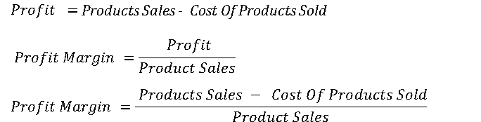
Now, let's say we want to create Calculated Measures that will calculate ProftMargin for the United kingdom Sales territory Region. Using the formula above this can be achieved with the logic below.

Listing 6:

'FactResellerSales'[ProftMargin_UK]:=
SUMX (
    FILTER ('FactResellerSales',
            'FactResellerSales'[SalesTerritoryKey] = 10
     ),
    ( ( 'FactResellerSales'[SalesAmount] - 'FactResellerSales'[TotalProductCost] ) / 
        'FactResellerSales'[SalesAmount]
     )
)

Here, the SUMX Iterator scans the FactResellerSales filtering the records to United kingdom Sales territory Region with  SalesTerritoryKey of 10. It then performs row-by-row calculations using the profit margin formula expression provided as the second argument.   After completing the row-by-row calculations, it then sums the partial results.

Various other functional groups can also be incorporated in the two iterator arguments making the very powerful in the hands of DAX developers who learn how to use them.

Iterator Performance

When coming from a SQL background, it is esp. easy to assume that Iterators ( e.g SUMX ) will be inherently slow compared to Aggregators (e.g SUM), because they perform calculations row by row.  On the contrary, no performance penalty is incurred by choosing iterators over aggregators.  Aggregators are just a different syntax version of iterators. The basic aggregation functions are just a shortened version of the corresponding X-suffixed function.

For example, consider the following expression:

SUM('FactResellerSales'[Freight])

Internally this gets translated to iterator version below:

SUMX('FactResellerSales', 'FactResellerSales'[Freight])

Therefore the only advantage in using SUM is that it is a shorter syntax with one simple argument.

Introduction to Logical functions

Functions that can make your life easier in writing complex algorithms are Logical Functions. If you are familiar with SQL Logical Functions the DAX counterparts work mostly the same. We will look at a few examples here but you can find the complete list of these functions here: DAX Logical functions.

IF Function

One of the helpful ones is the IF function. It checks if a condition provided as the first argument is met.

IF(<logical_test>,<value_if_true>[,<value_if_false>])

The statement above returns one value if the <logical_test> condition is TRUE, and returns another value if the condition is FALSE.

For instance, the Calculated Measure in listing 7 below checks the 'FactResellerSales'[Profit]  > 0 conditions and returns "Gain" or "Loss"

Listing 7:

'FactResellerSales'ProfitLossDesc :=
IF('FactResellerSales'[Profit]>0,"Gain","Loss")

Note that by using parentheses one can control the order and evaluation of many operators at a time. The example in Listing 8 below uses AND (&&) and OR (||) to test more than one condition.

Listing 8:

= IF([StateProvinceCode]<> "" && ([MaritalStatus] = "M" || [NumberChildrenAtHome]>0), [State])

Also, note that in Listing 8 no value has been specified for value_if_false, therefore, a default empty string is returned if false.

Nested IF

Nested IF statements are most useful because they allow you to evaluate various other conditions if a condition is FALSE as shown in Listing 9 below. 

'FactResellerSales'ProfitLossDesc := 
IF([Profit]>0,"Gain",IF([Profit]<0,"Loss","BreakEven"))

Nested IF  Vs  SWITCH

Simple nested IF is ok, but the logic could get complicated and difficult to read if there are many levels of nesting. If you are testing one condition with a lot of nesting it can be replaced with a more compact SWITCH Version.

For eg. the example in Listing 10 below is used to create a short WeekDay name in the DimDate dimension table using nested IF statements.

Listing 10:

'DimDate'[ShotWeekDayName] =
IF (
    [WeekNumber] = 1,
    "Sun",
    IF (
        [WeekNumber] = 2,
        "Mon",
        IF (
            [WeekNumber] = 3,
            "Tue",
            IF (
                [WeekNumber] = 4,
                "Wed",
                IF (
                    [WeekNumber] = 5,
                    "Thur",
                    IF (
                        [WeekNumber] = 6,
                        "Fri",
                        IF ( [WeekNumber] = 7, "Sat", "Unknown weekday" )
                    )
                )
            )
        )
    )
)

Listing 11 below shows a compact version using the SWITCH function.

Listing 11:

Listing 11:
'DimDate'[ShotWeekDayName] =
SWITCH (
    [WeekNumber],
    1, "Sun",
    2, "Mon",
    3, "Tue",
    4, "Wed",
    5, "Thur",
    6, "Fri",
    7, "Sat",
    "Unknown"
)

As we can see, the above SWITCH expression checks for only a single condition. A trick you can use to make the SWITCH function check multiple conditions in the same expression is to set the first condition to TRUE(). As noted earlier, SWITCH is converted into a set of nested IF functions where the first one that matches wins. By using TRUE as the first parameter means, you invariably test multiple conditions by asking SWITCH to return the first result where the conditional expression evaluates to TRUE.”

Listing 12:

'DimReseller'[ResellerGrade] =
 SWITCH (
   TRUE (),
  'DimReseller'[ProductLine] = "Touring" && 'DimReseller'[AnnualRevenue] >250000, "TouringStar",
  'DimReseller'[ProductLine] = "Mountain"  && 'DimReseller'[AnnualRevenue] >250000, "MountainStar",
  'DimReseller'[ProductLine] = "Road" && 'DimReseller'[AnnualRevenue] >250000, "RoadStar"
)

In the Calculated Column Listing12 above, SWITCH expression will return the first and only result where the conditional expressions evaluates to TRUE for each row.

IFERROR Function

In reports and dashboards, there is the need to detect error conditions in your DAX calculations and expressions before they unpleasantly show up. IFERROR is a useful function that can intercept such error and for instance replaces it with a blank, empty string "or appropriate values or texts.

Syntax

IFERROR(value, value_if_error)

Evaluates an expression and returns a specified value if the expression returns an error; otherwise returns the value of the expression itself.

In the example below, it is used as a wrap-around ProftMargin calculation to return blank if the calculation errors out as shown in Listing xxx below.

Listing 13:

'FactResellerSales'[ProftMargin]:=
IFERROR (
     SUMX (
          'FactResellerSales' ,
           ( 'FactResellerSales'[SalesAmount] -  'FactResellerSales'[TotalProductCost] )  /   
            'FactResellerSales'[SalesAmount]
     )
     , BLANK ()
)

If we did not use IFERROR and the SalesAmount column, for instance, contained a zero, the result would error out because if a single row generates a calculation error, the error propagates to the whole column. By using IFERROR, we intercept such errors and replace them with a blank value.

Introduction to Relational functions

This topic is quite advanced so do not worry if you don’t get it the first time, try and read on expanded table concept in Part I first if you are just joining the series.  There are two relational functions you can use in DAX calculations and expressions, namely, RELATED and  RELATEDTABLE. We will first explore their general behavior and then proceed to look at their syntax and how they are used.

Whenever one references a table in DAX, it is always the Expanded Table, as we learned in Part 1, table expansion takes place when a table is defined and the model built, not when the table is being queried.

The two functions we discuss here are not about how tables are joined. These are functions that are rather used to return a value or rows of values from related tables to be used in operations during row-by-row calculations.  The one you use depends on which side of one-to-many joins in a Tabular Model you are operating from.

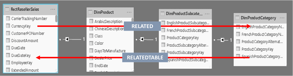
 Figure 6: Showing how the two relational functions enable you to traverse a model to related tables following a chained many-to-one relationship.

Figure 6 above shows a section of the Adventureworks model with chained joins starting from FactResellerSales reaching DimProductCategory through DimProduct and DimProductSubcategory. When you employ these functions, no matter how far a related table is removed from the original table, DAX will follow the chained relationships and returns the related value(s) needed.

RELATED

For instance, let's say we want to create a new column in FactResellerSales using an operation that involves values from DimProductCategory. To be able to do this we need to use the RELATED function. The RELATED function is used to access the one-side of the chained relationships from the many-side as indicated in figure 3 above. Because of this, only one row in related tables exists when you traverse the chain with the RELATED function. Note that If no row exists, RELATED returns a BLANK.

RELATEDTABLE 

If on the other hand, we want to create a new column in DimProductSubcategory using an operation that involves values from FactResellerSales then we need to use the RELATEDTABLE function. If an expression is on the one-side of the relationship and needs to access the many-side, because many rows from the many sides might be available for a single row, one has to traverse the chain using the RELATEDTABLE function. RELATEDTABLE returns a table containing all the rows related to the current row.

In summary, the two function are key DAX semantics that gives you access to the related columns of Expanded Tables in a Tabular Model and also tells the DAX engine how to traverse the model and return a value or rows of values during a row by row operations.

Intro: RELATED function

Below is the general syntax of the RELATED function. It Returns a related value from a column in another table.

RELATED(<Column Name>)

You specify the column that contains the data that you want, and the function follows an existing many-to-one relationship to fetch the value from the specified column in the related table.

So let's say we want to calculate Retail Amount in the FactResellerSales table as the product of OrderQuantity and ListPrice from the products table, Listing 14 shows how it can be achieved.

Listing 14:

'FactResellerSales'[RetailAmount] =
'FactResellerSales'[OrderQuantity] * RELATED('DimProduct'[ListPrice] )

If instead of a Calculated Column we would like to implement the same formula as a calculated measure, it will be as shown in Listing 15 below.

Listing 15:

'FactResellerSales'[RetailAmount]:=
  SUMX (
        'FactResellerSales',                                           
        'FactResellerSales'[OrderQuantity] * RELATED('DimProduct'[ListPrice] )
)

Note that in both Listing 14 and Listing 15 DAX perform row-by-row calculations, thus the need for The RELATED function to obtain values from related tables. By default, Calculated Column calculations are performed row-by-row as in Listing 14 and for the Calculated Measure in Listing 15, the SUMX iterator function also performs calculation row-by-row.

The next example Listing 16 below shows how RELATED has been used in a SWITCH statement to create a new adjusted price column based on percentages applied to specific Product Subcategories

Listing 16:

 'FactResellerSales'[AdjustedRetailPrice] =
SWITCH (
    RELATED ('DimProductSubcategory'[EnglishProductSubcategoryName]),
     "Mountain Bikes",   'FactResellerSales'[UnitPrice] * 0.98,
     "Road Bikes",       'FactResellerSales'[UnitPrice] * 0.93,
     "Touring Bikes",    'FactResellerSales'[UnitPrice] * 0.93,
     "Brakes",         'FactResellerSales'[UnitPrice] * 0.95,
     "Mountain Frames", 'FactResellerSales'[UnitPrice] * 0.95,
     'FactResellerSales'[UnitPrice]
)

In the final example in Listing 17 below, the complex iteration in Listing 16 above is modified to use the RELATED function to filter the FactResellerSales table using the related DimSalesTerritory Table.

Listing 17:

'FactResellerSales'[ProftMarginUK]:=
SUMX (
       FILTER ( 'FactResellerSales',
                RELATED('DimSalesTerritory'[SalesTerritoryRegion]) = "United Kingdom"
       ),
       ( ( 'FactResellerSales'[SalesAmount] - 'FactResellerSales'[TotalProductCost] ) /     
         'FactResellerSales'[SalesAmount] 
       )
)

Below are summary notes about the RELATED function

1. In all examples above there is an operation with a row-by-row level calculation where we traverse the model from the many-one side to get or check a related value.
2. The RELATED function needs a row context; ie where there is a row-by-row calculation.  Hence, it can be used only in one of the following cases -
   1. A calculated column expression.
   2. As a nested function in an expression that uses an iterator function, such as SUMX, etc.
   3. It allows you to traverse the model from many-side to any related tables on the one-side in the chain of many-to-one relations.
   4. When DAX RELATED function performs a lookup, it examines all values in the specified table regardless of any filters that may have been applied.

Note, it is OK if you don't grasp the meaning of the fourth point at this stage, it will become more apparent in the next installment of the series when we talk about interactive filtering and Evaluation Context.

Intro: RELATEDTABLE function

Below is the general syntax of the RELATEDTABLE function.

RELATEDTABLE(<Table>)

RELATEDTABLE returns a table containing all the rows related to the current row. It returns the related tables filtered so that it only includes the related rows.

For example, as shown in Listing 18 below, using RELATEDTABLE and iterators, we can create a Calculated Column that computes and stores sales per each product subcategory in the DimSubProductCategory table.

Listing 18:

'DimSubProductCategory'[CategorySales] =
SUMX (
    RELATEDTABLE ('FactResellerSales'),
    'FactResellerSales'[SalesAmount]
)

RELATEDTABLE function is used to pass the FactResellerSales table which is on the many-side of DimSubProductCategory in the chained relationship (as shown in figure 3 ) as the table argument for the SUMX iterator.

Listing 19 below creates a  Calculated Column in DimProductCategory table that stores the count of the related number of rows of products for each ProductCategory

Listing 19:

'DimProductCategory'[NumOfProducts] =
COUNTROWS(RELATEDTABLE(DimProduct))

RELATEDTABLE is used to pass the DimProduct table which is on the many-side of DimProductCategory in the chained relationship.

In the final example Listing 20 below creates a  Calculated Column in DimReseller table that stores the Biggest Order in terms of sales for each reseller by selecting the maximum sale value from the related  FactResellerSales table.

Listing 20:

'DimReseller'[BiggestOrder] =
MAXX(
     RELATEDTABLE('FactResellerSales'),
    'FactResellerSales'[SalesAmount]
)

Intro: RELATEDTABLE function

• It allows you to traverse the model from many-side to any related tables on the one-side in the chain of one-to-many  relations
• RELATEDTABLE and iterators are useful for creating Calculated Columns in Dimension tables. Because the column is calculated, this result is consolidated in the table, and it does not change according to the user selection in the report, as it would if it were written in a measure.

Scoping Complex Calculation

One very useful aspect of DAX is that it allows you to build more complex calculations using an existing one. We saw this in the previous section where complex algorithms can be broken down into simpler calculations using Query Measures and Query variables which were called and reused within the same Query. We can apply the same technique to Calculated Columns and Calculated Measures. When you create DAX Calculations in DAX models they are global in scope and thus can be called and used in any other calculations that have access to the model.

To implement the profit margin formula with reusable code to make it easy to understand the logic four separate Calculated Measure can be created to achieve that as shown in Listings 21- 24 below.  Listing 23 leverages two existing Calculated Measures  Listings 21 and Listings 22 to create profit which is then finally leveraged to create profit margin Measure.

Listing 21:

ProductsSales:=
        SUM ('FactResellerSales'[SalesAmount] )

Listing 22:

CostOfProductsSold :=
        SUM ('FactResellerSales'[TotalProductCost] )

Listing 23:

Profit:= [ProductsSales] - [CostOfProductsSold]

Listing 24:

ProfitMargin:=
        DIVIDE ([Profit],[ProductsSales] )

The beauty of this approach is each of these measures can be called and used in other calculations in any report with access to the model.

Using Variables to scope Calculation

Variables are a major feature that makes writing complex DAX code easier because you can use them to greatly increases the readability and reusability of your code in complex algorithms. Their use is very simple, in this example, they are used in Profit Margin calculations as shown in Listing 25 below:

Listing 25:

FactResellerSales[ProfitMargin] :=
VAR ProductsSales=
        SUM ('FactResellerSales'[SalesAmount] )     
VAR CostOfProductsSold =
        SUM ( 'FactResellerSales'[TotalProductCost] )      
VAR Profit = [ProductsSales] - [CostOfProductsSold]
VAR ProfitMargin = DIVIDE ( [Profit], [ProductsSales] )
RETURN
   ProfitMargin

From previous examples of similar calculations, you can already appreciate the advantage in terms of code readability. By assigning names to expressions, the code is simpler to read and maintain over time. Very useful if you have complex logic with not much reusable code outside of the logic.

Note that you can define variables with both scalar values and tables. There is no difference in the syntax or their usage. The next example creates a measure that calculates Sales for the Bikes Product Category as shown in Listing 26 below.

Listing 26:

Listing 26:
'FactResellerSales'[ProfitMargin_Bikes]:=
VAR BikeSales =            // Save the rows of Sales which are related Bikes
    FILTER(                 
        'FactResellerSales',
        RELATED ('DimProductCategory'[EnglishProductCategoryName] ) = "Bikes"
    )
VAR BikeProfit =           
    SUMX(                     // compute the profit for Bikes
        BikeSales,
        'FactResellerSales'[SalesAmount] - 'FactResellerSales'[TotalProductCost]
    )
VAR BikeProfitMargin = BikeProfit/'FactResellerSales'[SalesAmount]
RETURN
   BikeProfitMargin

As we can see, the Variable BikeSales is assigned to a table expression that saves the rows of Sales which are related to Bikes. This is passed over to the BikeProfit variable to be iterated over by a SUMX function.

We've used variables in Calculated Measures and queries, note that they also work perfectly well with Calculated Columns.

Intro: Variables

The VAR keyword introduces the definition of a variable.

• You can have as many variables as needed in a single expression, and each one has its own VAR definition.
• The RETURN keyword defines the expression to return as a result. Inside RETURN expression, you can use the variables, which are replaced by the computed value.

There is a lot more to variables than what we discussed here, besides helping you write complex and efficient calculations they can be used to improve your formulas such as; Improve performance, Improve readability, Simplify debugging, and Reduce complexity.

Other Function groups

With DAX, there are many functions available to shape, form, or otherwise analyze your data in Calculations that cannot be covered in this series. very useful ones are  Time-intelligence functions and Parent and Child functions. For the full reference list of function groups, you can follow this link.

Summary

We learned the general DAX syntax structures as one transition from writing DAX Queries to writing DAX formulas for use in Power BI reports. After that, we looked at how to create the two types of formulas, Calculated Column, and Calculated Measures outlining the major differences between the two. We proceeded to have an introductory look at few important DAX function groups very useful and often used in DAX formulas. We finally learned how to build more complex calculations through scoping techniques that use existing calculations and variables.

Take-away

The functions and functional groups introduced in this section form the basis for writing complex DAX calculations using Power BI formulas. Using these functions and scoping techniques, one can create a complex algorithm with DAX formulas that can be used in various Power BI reporting scenarios. Scoping complex calculation not only improves readability and reduce complexity, but it is also very useful for simplifying debugging and improve performance.

Next

In the next installment of the series, we are going to see how these calculations behave, esp. in response to user-actions when you use them in various types of reports.