This article is a guide on using SQL window functions in applications that need to make computational heavy queries. Data is proliferating at an astonishing rate. In 2022, the world produced and consumed 94 zetabytes of data. Today we have multiple tools like Hive and Spark to handle Big Data. Even though the tools differ in the types of problems they were designed to solve, they employ the fundamentals of SQL, which makes it slightly easier for people to work with big data. Window functions are an example of one such SQL concept. It is a must know for software engineers and data scientists.
SQL window functions are a powerful feature of SQL that allow users to perform calculations across a set of rows, or "window", in a query. These functions provide a convenient way to compute complex results using a simple, declarative syntax, and can be used to solve a wide range of problems.
PostgreSQL’s documentation does a good job introducing the concept:
A window function performs a calculation across a set of table rows that are somehow related to the current row. This is comparable to the type of calculation that can be done with an aggregate function. But unlike regular aggregate functions, use of a window function does not cause rows to become grouped into a single output row — the rows retain their separate identities. Behind the scenes, the window function is able to access more than just the current row of the query result.
Window Functions vs Aggregate Functions
Aggregate functions operate on a set of values and return a single scalar value. Some example of SQL aggregate functions are:
- AVG() - returns the average of a specified column values
- SUM() - returns the sum of all values
- MAX(), MIN() - returns the maximum and minimum value
- COUNT() - returns the total count of values
Aggregate functions are used with the GROUP BY clause which calculates the aggregate value for multiple groups in one query. Lets explain this with an example using sales transaction data from San Francisco and New York.
id  date        city           amount
1   2020-11-01  San Francisco   420.65
2   2020-11-01  New York       1129.85
3   2020-11-02  San Francisco  2213.25
4   2020-11-02  New York        499.00
5   2020-11-02  New York        980.30
6   2020-11-03  San Francisco   872.60
7   2020-11-03  San Francisco  3452.25
8   2020-11-03  New York        563.35
9   2020-11-04  New York       1843.10
10  2020-11-04  San Francisco  1705.00
We want to calculate the average daily transaction amount for each city. In order to calculate this we will need to group the data by date and city.
SELECT date, city, AVG(amount) AS avg_transaction_amount_for_city
FROM transactions
GROUP BY date, city;
The result of the above query is;
date       city          avg_transaction_amount_for_city
2020-11-01 New York      1129.85
2020-11-02 New York      739.65
2020-11-03 New York      563.35
2020-11-04 New York      1843.1
2020-11-01 San Francisco 420.65
2020-11-02 San Francisco 2213.25
2020-11-03 San Francisco 2162.425
2020-11-04 San Francisco 1705
The AVG() and GROUP BY aggregate functions gave us the average grouped by date and city. If you look at the rows, on Nov 2nd we had two transactions in New York and on Nov 3rd we had two transactions in San Francisco. The result set collapsed the individual rows by presenting the aggregate as a single row for each group.
Window functions like aggregate functions operate on a set of rows called a window frame. Unlike aggregate functions, window functions return a single value for each row from the underlying query. The window is defined using the OVER() clause. This allows us to define the window based on a specific column, similar to GROUP BY in aggregate functions. You can use aggregate functions with window functions but you will need to use them with the OVER() clause.
Lets explain this with an example using the transaction data above. We want to add a column with the average daily transaction value for each city. The window function below gets us the result.
SELECT id, date, city, amount,  AVG(amount) OVER (PARTITION BY date, city) AS  avg_daily_transaction_amount_for_city
FROM transactions
ORDER BY id;
This is the result:
id  date        city          amount      avg_daily_transaction_amount_for_city
1   2020-11-01  San Francisco 420.65      420.65
2   2020-11-01  New York      1129.85     1129.85
3   2020-11-02  San Francisco 2213.25     2213.25
4   2020-11-02  New York      499.00      739.65
5   2020-11-02  New York      980.30      739.65
6   2020-11-03  San Francisco 872.60      2162.425
7   2020-11-03  San Francisco 3452.25     2162.425
8   2020-11-03  New York      563.35      563.35
9   2020-11-04  New York      1843.10     1843.1
10  2020-11-04  San Francisco 1705.00     1705
See that the rows are not collapsed. There is one row for each transaction with the calculated averages in avg_daily_transaction_amount_for_city.
The diagram below illustrates the difference between Aggregate functions and Window functions.
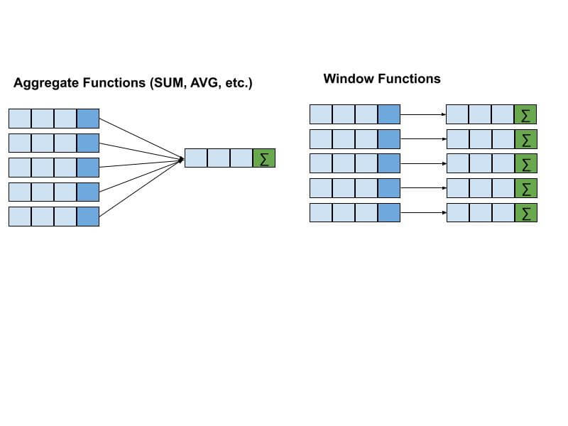
Similarities and differences between Window Functions and Aggregate Functions
Both window functions and aggregate functions:
- Operate on a set of rows
- Calculate aggregate amounts
- Group or partition data on one or more columns
Aggregate functions differ from window functions in:
- Using GROUP BY to define a set of rows for aggregation
- Group rows based on column values
- Collapses rows to a single row for each defined group
Window functions differ from aggregate functions in:
- Use OVER() instead of GROUP BY to define the set of rows
- Use more functions in addition to aggregates eg RANK(), LAG(), LEAD()
- Can group rows on the rows rank, percentile, etc. in addition to its column value
- Does not collapse rows to a single row per group
- Might use a sliding window frame based on the current row
Why use window functions?
A major advantage of window functions is it allows you to work with both aggregate and non-aggregate values all at once because the rows are not collapsed together. They also help with performance issues. For example, you can use a window function instead of doing a self join or a cross join.
Window function syntax
Lets walk through the syntax for window functions with a few examples. We will use the same dataset above which I have copied below.
date        city          avg_transaction_amount_for_city
2020-11-01  New York      1129.85
2020-11-02  New York      739.65
2020-11-03  New York      563.35
2020-11-04  New York      1843.1
2020-11-01  San Francisco 420.65
2020-11-02  San Francisco 2213.25
2020-11-03  San Francisco 2162.425
2020-11-04  San Francisco 1705
We want to calculate the running transaction total for each day in each city. The query below calculates that for you.
SELECT id, city,
       date,
       SUM(amount) OVER
         (PARTITION BY city ORDER BY date)
         AS running_total
  FROM transactions
The first part of the above aggregate, SUM(amount) looks like any other aggregation. Adding OVER, designates it as a window function. PARTITION BY narrows the window from the entire dataset to individual groups within the dataset. The above query groups by city and orders by date. Within each city group, it is ordered by date and the running total sums across the current row and all previous rows of the group. When the value of city changes, you will notice the value of running_total starts over for that city. This is the result of the above query.
id  city          date        running_total
1   New York      2020-11-01  1130
2   New York      2020-11-02  1870
3   New York      2020-11-03  2433
4   New York      2020-11-04  4276
5   San Francisco 2020-11-01  421
6   San Francisco 2020-11-02  2634
7   San Francisco 2020-11-03  4796
8   San Francisco 2020-11-04  6501
The ORDER BY and PARTITION define what is referred to as the window – the ordered subset of data over which calculations are made
Types of Window Functions
There are several types of SQL window functions, each with a different purpose and behaviour. Below is a list of all the window functions. I’ve linked to the Postgresql documentation if you are looking for more information on specific window functions that I do not cover:
- Aggregate functions: These functions compute a single value from a set of rows
- SUM(), MAX(), MIN(), AVG(). COUNT()
- Ranking functions: These functions assign a rank to each row in a partition
- RANK(), DENSE_RANK(), ROW_NUMBER(), NTILE()
- Analytic functions: These functions compute values based on a moving window of rows
- Offset functions: These functions allow users to retrieve values from a different row within the partition
- FIRST_VALUE() and LAST_VALUE().
More examples of using Window Functions
One of the main benefits of using SQL window functions is that they allow users to perform complex calculations without using a subquery or joining multiple tables. This can make queries more concise and efficient, and can improve the performance of the database.
Let's take a new example. The table below called train_schedule has the train_id , station and arrival time for trains in the San Francisco Bay Area. We need to calculate the time to the next station for each train in the schedule.
Train_id Station       Time
110      San Francisco 10:00:00
110      Redwood City  10:54:00
110      Palo Alto     11:02:00
110      San Jose      12:35:00
120      San Francisco 11:00:00
120      Redwood City  11:54:00
120      Palo Alto     12:04:00
120      San Jose      13:30:00
We can calculate this by subtracting the station times for a pair of contiguous stations for each train. Calculating this without window functions can be complicated. Most developers would read the table into memory and use application logic to calculate the values. The window function LEAD greatly simplifies this task.
SELECT
    train_id,
    station,
    time as "station_time",
    lead(time) OVER (PARTITION BY train_id ORDER BY time) - time
        AS time_to_next_station
FROM train_schedule
ORDER BY 1 , 3;
We create our window by PARTITIONING on the train_id and ordering the partition on the time (station time). The LEAD() window function obtains the value of a column for the next row in the window. We calculate the time to the next station by subtracting the window function lead time from the individual column time. The results are below.
train_id station       time        time_to_next_station
110      San Francisco 10:00:00    00:54:00
110      Redwood City  10:54:00    00:08:00
110      Palo Alto     11:02:00    01:33:00
110      San Jose      12:35:00    —
120      San Francisco 11:00:00    00:54:00
120      Redwood City  11:54:00    00:10:00
120      Palo Alto     12:04:00    01:26:00
120      San Jose      13:30:00    —
Building on the previous example, what if we had to calculate the elapsed time of the trip until the current station? You can use the MIN() window function to obtain the starting time for each window and subtract the current station time for each row in the window.
SELECT
    train_id,
    station,
    time as "station_time",
    time - min(time) OVER (PARTITION BY train_id ORDER BY time)
                                AS elapsed_travel_time,
    lead(time) OVER (PARTITION BY train_id ORDER BY time) - time
                                AS time_to_next_station
FROM train_schedule;
Our window doesn’t change. We still partition on train_id and order the window on time (station time). What changes is the calculation we perform for each row in the window. In the query above, we subtract the current rows time from the earliest rows time in the window, which happens to be the time the train left the first station. This gives us the elapsed time of the trip for each station.
Here is the result:
train_id station         time        elapsed_travel_time time_to_next_station
110      San Francisco   10:00:00    00:00:00            00:54:00
110      Redwood City    10:54:00    00:54:00            00:08:00
110      Palo Alto       11:02:00    01:02:00            01:33:00
110      San Jose        12:35:00    02:35:00            —
120      San Francisco   11:00:00    00:00:00            00:54:00
120      Redwood City    11:54:00    00:54:00            00:10:00
120      Palo Alto       12:04:00    01:04:00            01:26:00
120      San Jose        13:30:00    02:30:00            —
In conclusion, SQL window functions provide a convenient and efficient way to perform calculations across a set of rows in a query. These functions can be used to solve a wide range of problems in data analysis and manipulation, and can improve the performance of the database.