

Introduction
TOP is one of the many syntactical operators available in T-SQL and at a first view, it could seem very simple and not particularly interesting. According to the official documentation, it “limits the rows returned in a query result set to a specified number of rows or percentage of rows”.
The following is the syntax for SQL Server and Azure SQL Database:
[

TOP (expression) [PERCENT]

[ WITH TIES ]

]
TOP has several characteristics that are worth mentioning:
- It is not an ANSI standard operator
- If you specify PERCENT, the expression argument is converted to the FLOAT data type. Otherwise the argument is converted to a BIGINT; in any case the argument must be greater or equal to zero
- It can be used without the ORDER BY clause. In this case you, do not know to which order the results of the TOP are related
- It always runs in a serial zone of the execution plan
In this article, I am going to dig into two interesting scenarios. The first one is when the TOP argument is small enough to leverage the Row Goal. The second one is when it is big enough to ensure no rows are cut from the results, where we will see this can be used as a powerful tuning tool.
Notes
- I have carried out all the scripts on SQL Server 2019 CTP 2.5
- All the examples, with the exception of the last one, are based on AdventureWorks database with the addition of two tables (Sales.SalesOrderHeaderEnlarged and Sales.SalesOrderDetailEnlarged) created by the Jonathan Kehayas’ script that you can find here. The last example is self-consistent and database independent.
- I am often going to use a particular number: 2147483647 (231-1). This is the maximum for the INT data type, and it is supposed to be higher than the cardinality of each table I will refer to. If you think that it is not big enough for your environment, you could use the maximum for the BIGINT data type and for sure, you will not have a table with such number of rows: 9223372036854775807 (263-1)
The Row Goal
Referring to the official documentation, we know that “when the Query Optimizer estimates the cost of a query execution plan, it usually assumes that all qualifying rows from all sources have to be processed. However, some queries cause the Query Optimizer to search for a plan that will return a smaller number of rows faster”.
If you want to limit the number of the returned rows specifying the target number, you can use one of the specific keywords listed below.
- TOP, IN or EXISTS clauses
- FAST number_of_rows query hint
- SET ROWCOUNT number_of_rows statement
In this case, and if other conditions that we will see later are observed, the Query Optimizer (QO) can leverage the “Row Goal”, that basically is an optimization strategy.
As an example, take a look at the following query and its plan:
select top 10 * from Production.Product;
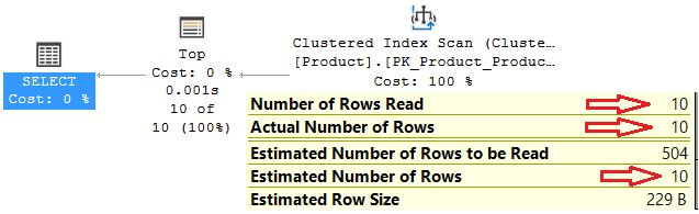
Fig. 1
At a first view, one could think that the Clustered Index Scan operator performs a scan of the whole table and then the TOP operator cuts all the rows except the first ten. Actually, as it is clear from the tooltip, the Clustered Index Scan is aware that only ten records are requested. Therefore, the number of rows that are read and the cost of the whole query are reduced.
When the Row Goal is applied, the QO usually chooses non-blocking operators (nested loop joins, index seeks and lookups) instead of blocking operators (sort and hash).
Is there the Row Goal in the plan?
Starting from SQL Server 2014 SP3, SQL Server 2016 SP2, and SQL Server 2017 CU3, we have the new EstimateRowsWithoutRowGoal attribute for each operator of the plan affected by the Row Goal. It returns the number of rows that would have been estimated if the Row Goal were not applied.
For the versions of SQL Server prior to the ones mentioned above, it is not evident if the Row Goal is acting, but in this case we have at least two clues. The first one is about the Estimated Number of Rows for a scan of a table; if we see that there is not any residual predicate and that the Estimated Number of Rows is less than the cardinality of the table, then the Row Goal could be applied.
The second clue is when the following condition is true:
Estimated Operator Cost < (Estimated I/O Cost + Estimated CPU Cost) * Estimated Number of Executions
Although basically the Row Goal is an optimization strategy, in several circumstances it leads to an inefficient query plan. Very often, this is due to a higher number of rows to manage at runtime than expected or to an adverse data distribution.
In these situations, one possible workaround is to disable the Row Goal with the query hint, DISABLE_OPTIMIZER_ROWGOAL, available from SQL Server 2016 SP1, or the trace flag, 4138.
Final considerations
I would like to underline a couple of important aspects related to the Row Goal. The first one is that different Row Goals can be applied in different sections of the plan. Think for example about a query with several CTEs, each one with its own TOP clause.
The second one is that the Row Goal is applied when the ‘goal’ is less than the regular estimate; moreover, the Row Goal affects the optimizer choices, if there are any! If there are not more than one choice, the Row Goal is not applied.
From here, it should be clear that the only presence of TOP, FAST, IN, EXISTS in a query or ROWCOUNT in a script does not ensure the Row Goal.
A Tuning Tool
T-SQL is a declarative language. This means that the user enters code and lets the engine take care of choosing the best control flow to get the result. In short, writing the code, we express WHAT we want to do but not HOW to do; this is the QO’s job.
Using the TOP operator, there is the possibility to keep control of several choices of the QO and to address them towards the desired direction. In this sense, we can consider TOP as a tuning tool.
A First Example
As a first demonstrative example, look at the following queries. They logically do the same thing, but actually, they are very different although they give the same result.
SELECT
      BusinessEntityID
    , PersonType
    , FirstName
    , LastName
    , ModifiedDate
FROM  Person.Person
WHERE BusinessEntityID = 10000;
SELECT *
FROM
       (
           SELECT TOP 2147483647
                  BusinessEntityID
                , PersonType
                , FirstName
                , LastName
                , ModifiedDate
           FROM   Person.Person
       ) AS t
WHERE  BusinessEntityID = 10000;
These are the two related plans:
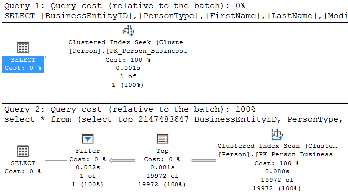
Fig. 2
The first one performs a Clustered Index Seek, 3 logical reads and ends in 2 ms; the second one performs a Clustered Index Scan, 3821 logical reads and ends in 184 ms.
What produces such a different plan in the second query is the presence of TOP in the derived table. The QO can foresee, using the statistics, the number of rows that will be extracted and that this number will probably be less than 2147483647, but it must guarantee not to go beyond that number. Therefore, at the beginning it performs a full scan and then, if it has more rows than requested, it applies the TOP criteria and only afterwards activates the filter of the WHERE condition.
The change done in this example has worsened the performance, but this is not the point. The important thing to understand is that the usage of the TOP operator inside a derived table forces the QO to change the shape of the original plan.
In the next sections, we will see several examples of how TOP can be helpful during the query tuning.
Join order
When we write a query with several joined tables, probably we write the join chain in a way that seems logical to us, but when we look at the query plan, very often we are surprised by the QO choices. Every T-SQL developer has asked himself if changes in the join order of the query can produce some modifications in the plan. Well, they do not.
All the following queries have the same plan, nevertheless the different join order, the usage of derived tables or CTEs:
--Original query

SELECT
               o.OrderDate
             , o.PurchaseOrderNumber
             , od.OrderQty
             , c.TerritoryID
FROM
               Sales.SalesOrderHeader AS o
    INNER JOIN Sales.SalesOrderDetail AS od
        ON o.SalesOrderID = od.SalesOrderID
    INNER JOIN Sales.Customer AS C
        ON o.CustomerID   = c.CustomerID
WHERE
               o.OrderDate       = '2011-05-31'
               AND c.TerritoryID = 6;

--Join order changed
SELECT
               o.OrderDate
             , o.PurchaseOrderNumber
             , od.OrderQty
             , c.TerritoryID
FROM
               Sales.Customer AS C
    INNER JOIN Sales.SalesOrderHeader AS o
        ON o.CustomerID   = c.CustomerID
    INNER JOIN Sales.SalesOrderDetail AS od
        ON o.SalesOrderID = od.SalesOrderID
WHERE
               o.OrderDate       = '2011-05-31'
               AND c.TerritoryID = 6;

--With a derived table
SELECT
               x.OrderDate
             , x.PurchaseOrderNumber
             , x.OrderQty
             , c.TerritoryID
FROM
               (
                   SELECT
                                  o.OrderDate
                                , o.PurchaseOrderNumber
                                , od.OrderQty
                                , o.CustomerID
                   FROM
                                  Sales.SalesOrderHeader AS o
                       INNER JOIN Sales.SalesOrderDetail AS od
                           ON o.SalesOrderID = od.SalesOrderID
               ) AS x
    INNER JOIN Sales.Customer AS C
        ON x.CustomerID = c.CustomerID
WHERE
               x.OrderDate       = '2011-05-31'
               AND c.TerritoryID = 6;

--With a Cte
;
WITH x
AS (SELECT
                   o.OrderDate
                 , o.PurchaseOrderNumber
                 , od.OrderQty
                 , o.CustomerID
    FROM
                   Sales.SalesOrderHeader AS o
        INNER JOIN Sales.SalesOrderDetail AS od
            ON o.SalesOrderID = od.SalesOrderID)
SELECT
               x.OrderDate
             , x.PurchaseOrderNumber
             , x.OrderQty
             , c.TerritoryID
FROM
               x
    INNER JOIN Sales.Customer AS C
        ON x.CustomerID = c.CustomerID
WHERE
               x.OrderDate       = '2011-05-31'
               AND c.TerritoryID = 6;
The following is the plan related to all of them:
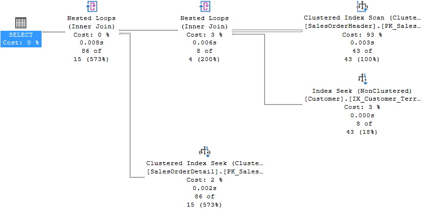
Fig. 3
As we can see, the QO joins SalesOrderHeader with Customer first and then it joins the result with SalesOrderDetails.
Now, imagine for a moment that for tuning reasons we wanted to see if joining SalesOrderHeader with SalesOrderDetails first could produce a better plan. It is possible to do it by using a join hint, maintaining the “Nested Loop” join type.
SELECT
                    o.OrderDate
                  , o.PurchaseOrderNumber
                  , od.OrderQty
                  , c.TerritoryID
FROM
                    Sales.SalesOrderHeader AS o
    INNER LOOP JOIN Sales.SalesOrderDetail AS od
        ON o.SalesOrderID = od.SalesOrderID
    INNER JOIN      Sales.Customer AS C
        ON o.CustomerID   = c.CustomerID
WHERE
                    o.OrderDate       = '2011-05-31'
                    AND c.TerritoryID = 6;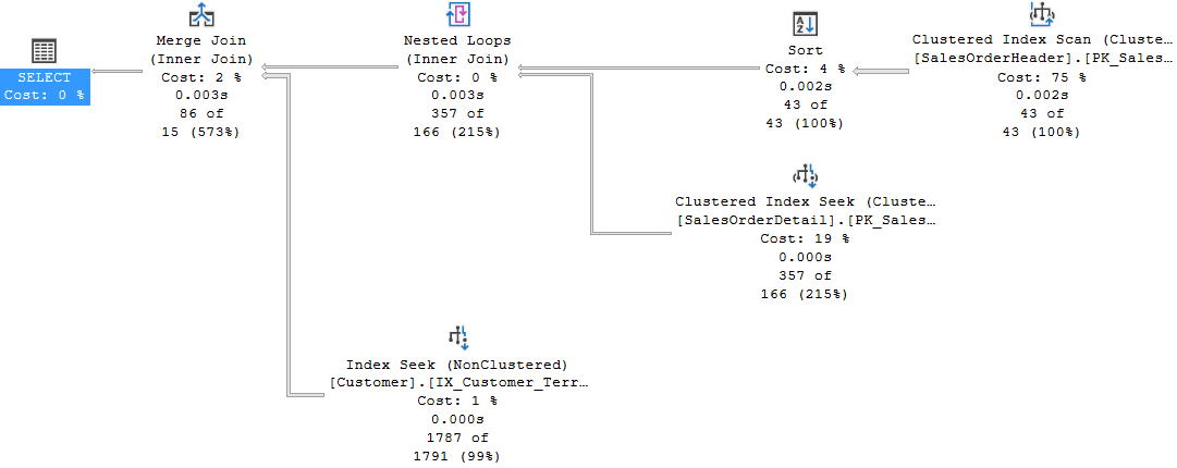
Fig. 4
In this way, we have reached the goal to change the join order, but this solution has two drawbacks. The first one is that we have forced the QO to use a loop join and it will never be free to change this type of join even if the statistics and the data distribution should change.
The second drawback is that a single join hint enforces the join order of the entire query. We do not want this. We want to join two tables first considering them as a single block leaving the QO free to join this block and the other tables as it wants.
The TOP operator can help to reach our goal.
;WITH x
AS (SELECT         TOP 2147483647
                   o.OrderDate
                 , o.PurchaseOrderNumber
                 , od.OrderQty
                 , o.CustomerID
    FROM
                   Sales.SalesOrderHeader AS o
        INNER JOIN Sales.SalesOrderDetail AS od
            ON o.SalesOrderID = od.SalesOrderID)
SELECT
               x.OrderDate
             , x.PurchaseOrderNumber
             , x.OrderQty
             , c.TerritoryID
FROM
               x
    INNER JOIN Sales.Customer AS C
        ON x.CustomerID = c.CustomerID
WHERE
               x.OrderDate       = '2011-05-31'
               AND c.TerritoryID = 6;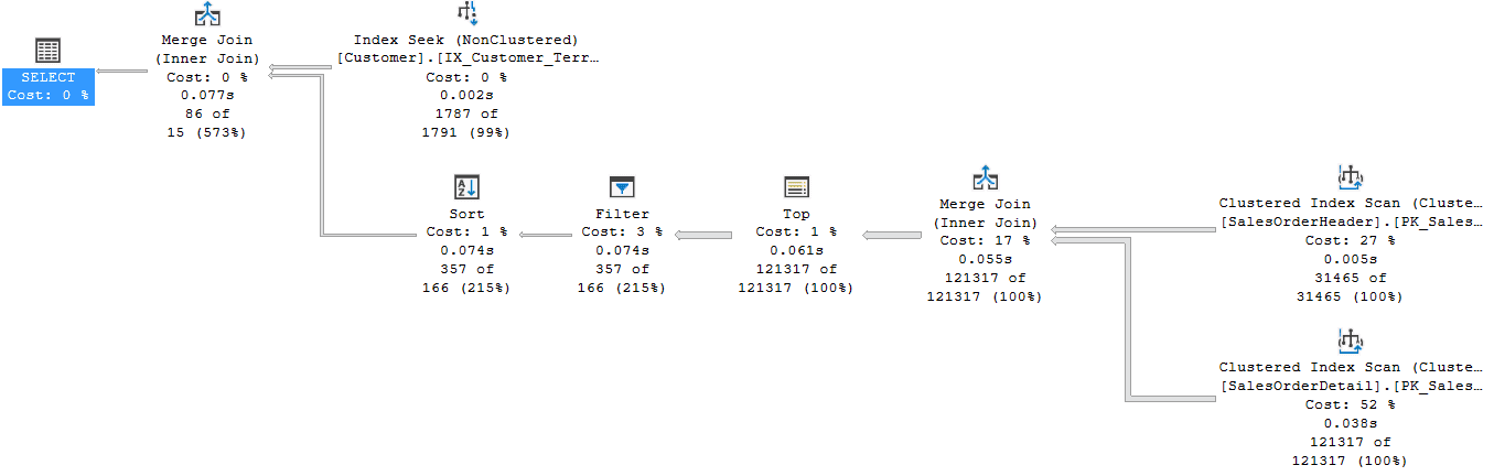
Fig. 5
The TOP operator in the CTE forces the QO to join the SalesOrderHeader and SalesOrderDetails first. This solution is better than the previous one because we do not have the two drawbacks anymore. Obviously, we can apply the same technique also in the derived table version of the query.
Join Type
With the same technique, it is possible to try changing the type of join chosen by the QO in order to see if a different one can help to improve the performance. As an example, carry out the following query:
SELECT
               p.ProductSubcategoryID
             , d.SalesOrderID
             , d.SalesOrderDetailID
             , d.CarrierTrackingNumber
FROM
               Production.Product AS p
    INNER JOIN Sales.SalesOrderDetail AS d
        ON d.ProductID = p.ProductID
           AND d.ModifiedDate
           BETWEEN '20111201' AND '20111228';
It ends in 128 ms using the Hash Match operator.
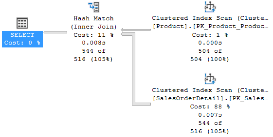
Fig. 6
Now, suppose that we wanted to see if the performance would benefit from a Merge Join instead of the Hash Match. One essential condition for the usage of the Merge Join is to have the two sets of data ordered in the same way. Since the Product table is read with a scan of the clustered index that is ordered by ProductId, the idea is to substitute the table SalesOrderDetail with a derived table where the data are ordered in the same way.
The TOP operator is essential for the usage of the ORDER BY clause inside the derived table. The following is the new query version and its plan:
SELECT
        p.ProductSubcategoryID
      , d.SalesOrderID
      , d.SalesOrderDetailID
      , d.CarrierTrackingNumber
FROM
        Production.Product AS p
    INNER JOIN
        (
            SELECT   TOP 2147483647
                     SalesOrderID
                   , SalesOrderDetailID
                   , CarrierTrackingNumber
                   , ProductID
            FROM     Sales.SalesOrderDetail
            WHERE
                     ModifiedDate
            BETWEEN  '20111201' AND '20111228'
            ORDER BY ProductID
        ) AS d
        ON d.ProductID = p.ProductID;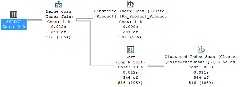
Fig. 7
In this way, the QO has chosen the Merge Join instead of the Hash Join and the query ends in 120 ms.
What if we wanted to test the Nested Loop join? We only have to cheat the QO making it believe that the derived table has very few rows. Once again, we can do it using the TOP operator with a variable in order to decouple the compilation from the execution.
DECLARE @i INT = 2147483647;
SELECT
        p.ProductSubcategoryID
      , d.SalesOrderID
      , d.SalesOrderDetailID
      , d.CarrierTrackingNumber
FROM
        Production.Product AS p
    INNER JOIN
        (
            SELECT   TOP (@i)
                     SalesOrderID
                   , SalesOrderDetailID
                   , CarrierTrackingNumber
                   , ProductID
            FROM     Sales.SalesOrderDetail
            WHERE
                     ModifiedDate
            BETWEEN  '20111201' AND '20111228'
            ORDER BY ProductID
        ) AS d
        ON d.ProductID = p.ProductID
OPTION (OPTIMIZE FOR (@i = 1));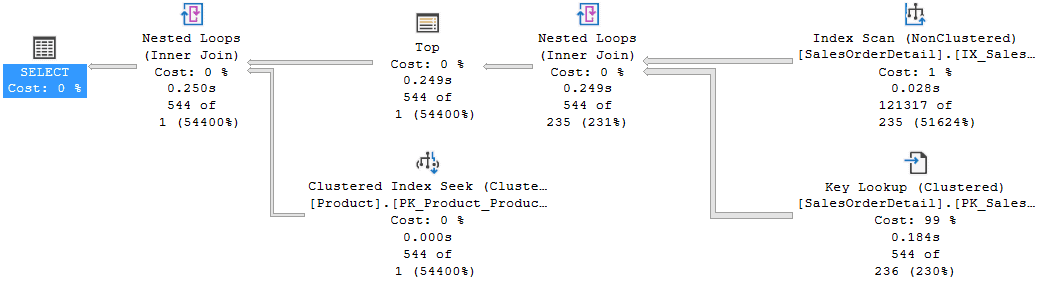
Fig. 8
As it was foreseeable, the performance has worsened substantially (309 ms) but it is without any doubt an interesting example of the usage of TOP operator with a variable.
Breakdown
When dealing with a complex query that is not particularly fast with several joins that involve tables, CTEs, or derived tables, one possible useful technique to speed up the execution is to break the query into multiple queries and materialize the intermediate result sets into temporary tables. In this way, SQL Server has the possibility to manage smaller plans with more affordable statistics related to the intermediate sets of data.
As we saw above, the TOP operator is a way to break down a query in memory, even if in general the materialization is more efficient and not always this technique gets the desired result in terms of performance. The following is a demonstrative example.
SELECT
               h.OrderDate
             , h.Status
             , d.OrderQty
             , d.UnitPrice
             , c.rowguid
             , c.ModifiedDate
             , t.TerritoryID
             , t.Name
             , crc.CardNumber
             , PrName = p.Name
             , p.ListPrice
             , sc.Name
             , cat.Name
             , m.Name
             , m.Instructions
             , st.Name
             , cat.Name
             , d.ProductID
FROM
               Sales.SalesOrderHeaderEnlarged AS h
    INNER JOIN Sales.SalesOrderDetailEnlarged AS d
        ON h.SalesOrderID         = d.SalesOrderID
    INNER JOIN Sales.Customer AS C
        ON c.CustomerID           = h.CustomerID
    INNER JOIN Sales.Store AS st
        ON st.BusinessEntityID    = c.StoreID
    INNER JOIN Sales.SalesTerritory AS t
        ON t.TerritoryID          = CASE h.SalesOrderID % 3
                                        WHEN 0 THEN
                                            1
                                        WHEN 1 THEN
                                            2
                                        WHEN 2 THEN
                                            5
                                        ELSE
                                            10
                                    END
    INNER JOIN Sales.CreditCard AS crc
        ON crc.CreditCardID       = h.CreditCardID
    INNER JOIN Production.Product AS p
        ON p.ProductID            = d.ProductID
    INNER JOIN Production.ProductSubcategory AS sc
        ON p.ProductSubcategoryID = sc.ProductSubcategoryID
    INNER JOIN Production.ProductCategory AS cat
        ON cat.ProductCategoryID  = sc.ProductCategoryID
    INNER JOIN Production.ProductModel AS m
        ON m.ProductModelID       = p.ProductModelID
WHERE
               d.OrderQty                                > 12
               AND DATEDIFF(DAY, h.OrderDate, h.DueDate) < 100
               AND d.ProductID                           = 712;
The above query takes an average of 1230 ms to complete. In order to break down this query, I am going to use a derived table; it gathers the tables Sales.SalesOrderHeaderEnlarged, Sales.SalesOrderDetailEnlarged and their related WHERE conditions. The following query does logically the same thing and extracts the same rows. It takes an average of 630 ms that means it is more or less 50% faster than the previous one.
SELECT
               h.OrderDate
             , h.Status
             , h.OrderQty
             , h.UnitPrice
             , c.rowguid
             , c.ModifiedDate
             , t.TerritoryID
             , t.Name
             , crc.CardNumber
             , PrName = p.Name
             , p.ListPrice
             , sc.Name
             , cat.Name
             , m.Name
             , m.Instructions
             , st.Name
             , cat.Name
             , h.ProductID
FROM
               (
                   SELECT         TOP 2147483647
                                  h.OrderDate
                                , h.Status
                                , h.CustomerID
                                , h.SalesOrderID
                                , h.CreditCardID
                                , d.OrderQty
                                , d.UnitPrice
                                , d.ProductID
                   FROM
                                  Sales.SalesOrderHeaderEnlarged AS h
                       INNER JOIN Sales.SalesOrderDetailEnlarged AS d
                           ON h.SalesOrderID = d.SalesOrderID
                   WHERE
                                  DATEDIFF(DAY, h.OrderDate, h.DueDate) < 100
                                  AND d.OrderQty                        > 12
                                  AND d.ProductID                       = 712
               ) AS h
    INNER JOIN Sales.Customer AS C
        ON c.CustomerID           = h.CustomerID
    INNER JOIN Sales.Store AS st
        ON st.BusinessEntityID    = c.StoreID
    INNER JOIN Sales.SalesTerritory AS t
        ON t.TerritoryID          = CASE h.SalesOrderID % 3
                                        WHEN 0 THEN
                                            1
                                        WHEN 1 THEN
                                            2
                                        WHEN 2 THEN
                                            5
                                        ELSE
                                            10
                                    END
    INNER JOIN Sales.CreditCard AS crc
        ON crc.CreditCardID       = h.CreditCardID
    INNER JOIN Production.Product AS p
        ON p.ProductID            = h.ProductID
    INNER JOIN Production.ProductSubcategory AS sc
        ON p.ProductSubcategoryID = sc.ProductSubcategoryID
    INNER JOIN Production.ProductCategory AS cat
        ON cat.ProductCategoryID  = sc.ProductCategoryID
    INNER JOIN Production.ProductModel AS m
        ON m.ProductModelID       = p.ProductModelID;
From the Field
Some months ago, I had to face a problem with a query that broke. The following code reconstructs the situation that is not particularly brilliant from the point of view of the table design.
We have the table T1, with the column RecValue (VARCHAR type) whose content can be a simple alphanumeric string or a string representation of a “date” or of a “number”. The table T1 has a reference to table T2, where there is the ContentType column that indicates the type of data contained in T1.RecValue. The allowed values of ContentType are ‘D’ that stands for Date, ‘N’ for Number and ‘C’ for Character.
The following script inserts three records in T1, each one referencing a different record in table T2 and with a content congruent with the ContentType value.
CREATE TABLE T2
(   Id          INT     NOT NULL PRIMARY KEY
  , ContentType CHAR(1) NOT NULL
  , CONSTRAINT Chk_ContentType CHECK (ContentType IN ( 'C', 'D', 'N' )));
GO

CREATE TABLE T1
(   Id       INT         IDENTITY(1, 1) PRIMARY KEY
  , TypeId   INT         NOT NULL
  , RecValue VARCHAR(50) NULL
  , CONSTRAINT Fk_T2 FOREIGN KEY (TypeId) REFERENCES T2 (Id));
GO

INSERT INTO T2 VALUES (1, 'C'), (2, 'D'), (3, 'N');
GO

INSERT INTO T1 VALUES (1, 'ABC'), (2, '2019-02-28'), (3, '12.3');
GO
The aim of the author of the query below is to FIRST select all the records that contain numeric values in T1.RecValue according to T2.ContentType and THEN cast T1.RecValue into a DECIMAL data type, filtering only those records that have that value higher than 10.
SELECT         NumericValue = CAST(T1.RecValue AS DECIMAL(17, 2))
FROM
               T1
    INNER JOIN T2
        ON T1.TypeId = T2.Id
WHERE
               T2.ContentType                          = 'N'
               AND CAST(T1.RecValue AS DECIMAL(17, 2)) > 10;
Unfortunately for the author, the QO’s strategy is different; it performs a Clustered Index Scan (look at the Estimated Plan in Fig. 9) with a predicate that carries out the cast into DECIMAL (Fig. 10) for every record of the table. Only after the scan, it joins with the records of the table T2 that have ‘N’ in ContentType.
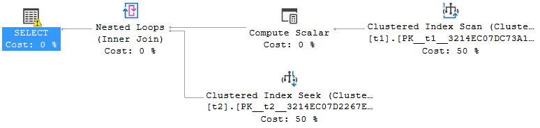
Fig. 9
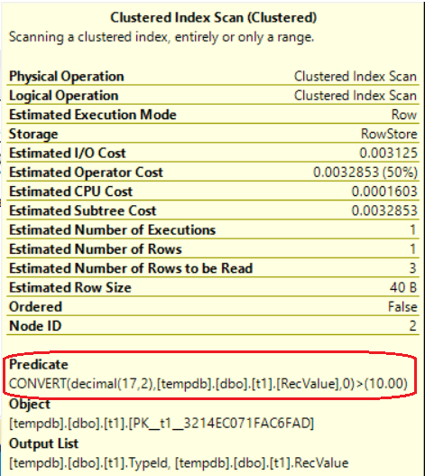
Fig. 10
The result is that as soon as the scan of table T1 encounters a value that cannot be converted into DECIMAL, the query breaks giving the following error: “Error converting data type varchar to numeric”.
The solution has been to rewrite the query forcing the QO FIRST to filter the records that should have numeric values in RecValue field and THEN comparing that value, casted into DECIMAL, with 10. All this has been possible thanks to TOP operator:
SELECT NumericValue = CAST(x.RecValue AS DECIMAL(17, 2))
FROM
       (
           SELECT         TOP 2147483647
                          T1.RecValue
           FROM
                          T1
               INNER JOIN T2
                   ON T1.TypeId = T2.Id
           WHERE          T2.ContentType = 'N'
       ) AS x
WHERE  CAST(x.RecValue AS DECIMAL(17, 2)) > 10;
The following is the related plan:
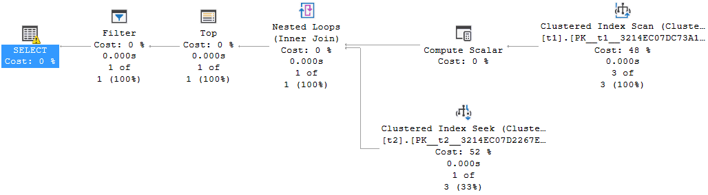
Fig. 11
In this plan, the Compute Scalar operator that follows the Clustered Index Scan represents the conversion into DECIMAL but actually it only defines the formula and it does not compute it. The calculation is performed only when the plan needs the result of it; this happens in the Filter operator that is AFTER the join with table T2. For this reason, the query ends without any error.
Conclusion
As a matter of fact, we can consider the TOP operator as a powerful tuning tool. It can be crucial in several situations but also useless or even damaging in others. For this reason, I would recommend to test a lot before using the techniques shown above in a production environment.
If you want to read more on these topics, my suggestion is to have a look at the following two cool and very interesting resources: an article written by Paul White and a video by Adam Machanic.
