Introduction

Big data consists of very large datasets, which can be structured, unstructured, and semi-structured. Data may be coming from various data sources in real-time or in batches. The traditional tools and technologies we have used in the past are not capable of processing and storing all this data in an efficient way. We need to have alternative tools and technologies to handle Big Data.

Azure Data Explorer is a PaaS resource from Azure which is ideal for analyzing large volumes of diverse data from any data source. In this article, I will discuss about the concepts and features of Azure Data Explorer (ADX), as well as the step-by-step process for creation and use of ADX.

About Azure Data Explorer

Azure Data Explorer is a fast and highly scalable data exploration service. It supports analysis of high volumes of heterogeneous data (structured and unstructured). It can scale quickly to terabytes of data. It can combine with other Azure services to provide end-to-end data analytics solution. The Azure Data Explorer workflow contains three major steps:

1. Create Database
2. Data Ingestion
3. Query the Data

I will discuss the workflow here in a demo scenario.

Step 1 - Create a Resource

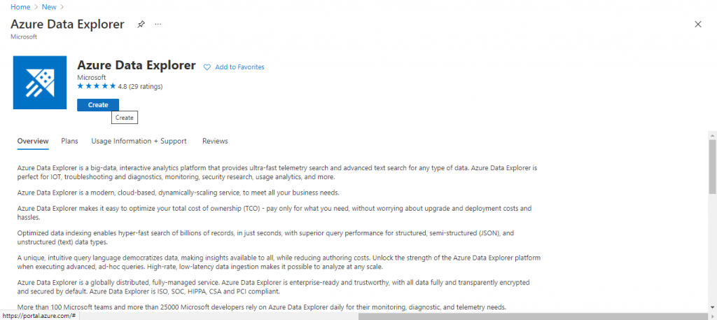
First, we need to search for Azure Data Explorer and create a resource. I login to the portal and search for the resource named Azure Data Explorer (ADX). I press the 'Create' button.

Step 2 - Create an ADX Cluster

In an Azure Data Explorer deployment, there are two services that work together: the Engine service and the Data Management (DM) service. Both the services are deployed as clusters of compute nodes or virtual machines.

The Engine service handles the processing of the incoming raw data and serves user queries. The Engine service is similar to the relational data model. There is a cluster at the top of the hierarchy. There can be multiple databases under a cluster. There are multiple tables and stored functions in each of the databases. Each table has a defined schema.

The DM service is responsible for connecting the Engine to the various data pipelines, orchestrating and maintaining continuous data ingestion process from these pipelines. The DM Service is optional.

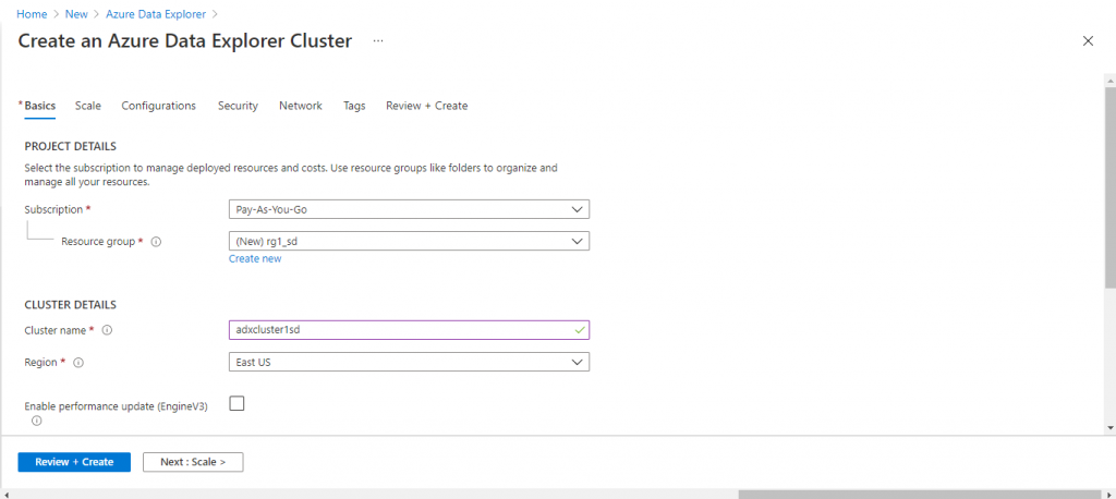
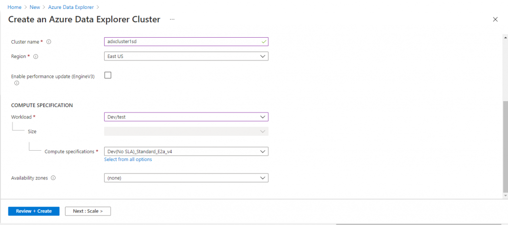
I need to create the ADX cluster first. In the Basics tab, I provide the required information. I keep most of the default options. I select the workload as Dev/Test and uncheck the EngineV3 option. That will keep the cost to a minimum. Based on the requirements, I may need to change these options later. I go to the other tabs and keep the default options for different parameters. In the 'Review + Create' tab, I press the 'Create' button.

Step 3: Database creation

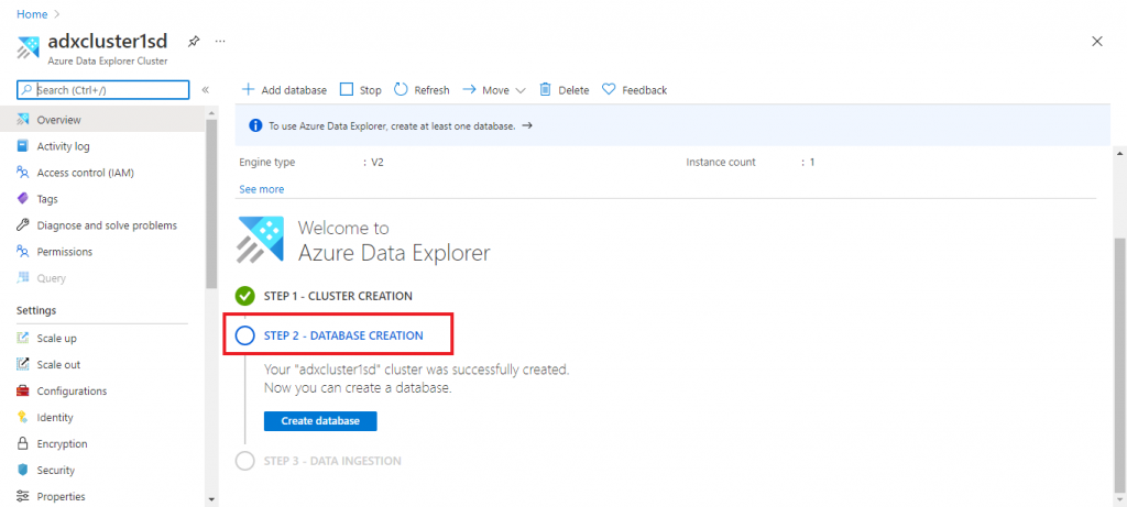
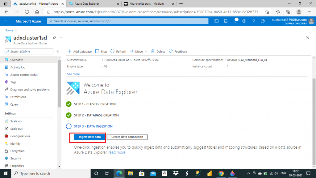
The ADX cluster creation takes some time. Once completed, I open the Overview page of the cluster. As the next step, I need to create a database. I press the 'Create Database' button. A pop-up window opens where I need to provide the details about the database to be created. I give a name for the database. I keep the Retention days and cache period values to 2 and 1 respectively to minimize the cost. These parameter values should be supplied as per your requirements.

At the end, I press the 'Create' button.

Step 4: Data Ingestion

Now the ADX cluster and database creation steps are completed. The third step is data ingestion. There are two options for data ingestion. I go for the quick option for data ingestion and press the 'Ingest New Data' option.

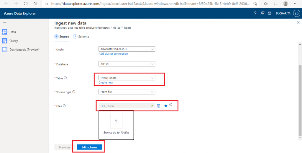
In the next screen, I need to give a name for the table where the data can be ingested in the selected database. I create a new table here. Alternatively, I may select an existing table as well for data loading. Next, I need to select the data source type from a dropdown list. I select the source as a file. Then, I need to select the file after browsing the folder structure. I may attach up to 10 files here. I attach a file, named FILE_LS.csv, from the local drive. At the end,

I press the 'Edit Schema' button.

A Data Ingestion basics need to be described. There are two types of ingestion based on the nature of data.

1. Batching Ingestion: This is most preferred and efficient type of ingestion. Here, data is ingested in batches and high ingestion throughput is achieved.
2. Streaming Ingestion: This is for real-time data which may flow continuously from the source. This type of ingestion allows near-real time latency for small sets of data per table.

The flow of data ingestion happens in few steps, detailed below:

• First, the input data is pulled from the data sources
• Data is batched or streamed to the Data Manager component of ADX
• Data Manager does the initial validation of the data and convert the data formats as required
• Schema matching is done with the existing table schema where the data needs to be mapped.
• Indexing, encoding, compression are also done on the ingested data.
• Data is persisted in the storage as per the retention policy
• Finally, Data Manager makes the data available to the Engine for query service.

All the data ingested into the tables are partitioned into horizontal slices or shards. Each shard contains few million records. Records in each shard are encoded and indexed. Shards are distributed in different cluster nodes for efficient processing. Also, data is cached in local SSD and memory based on the caching policy selected at the time of cluster creation. The query engine executes highly distributed and parallel queries on the dataset for the best performance.

Step 5: Start Ingestion

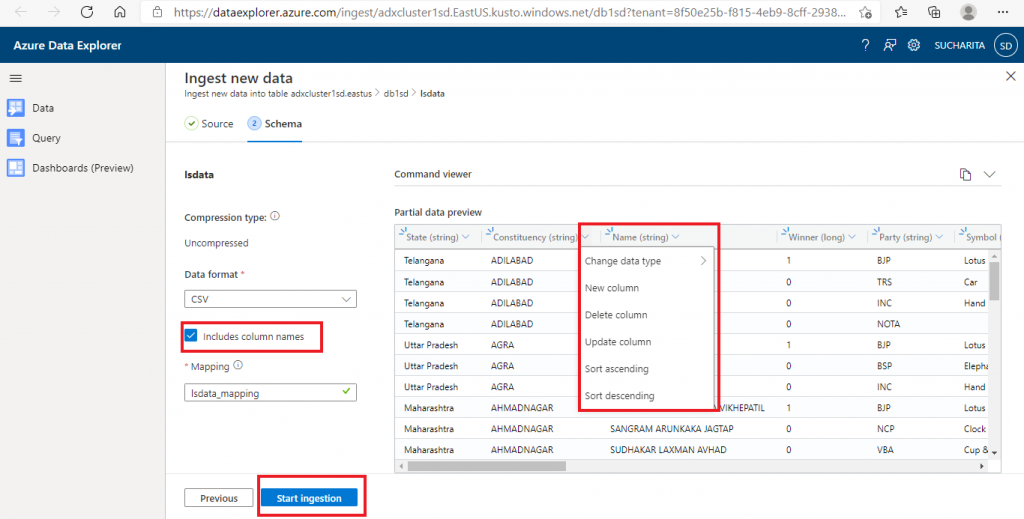
In the next screen, the table schema is created automatically from the data file supplied. The column names and data types are created based on the file columns and their values. It is possible to create, modify or delete any column in this screen. The data type of a column also can be changed as per your requirements. This column mapping of the file data and table structure is given a name. At the end, I press the 'Start Ingestion' button.

Step 6: Query the data

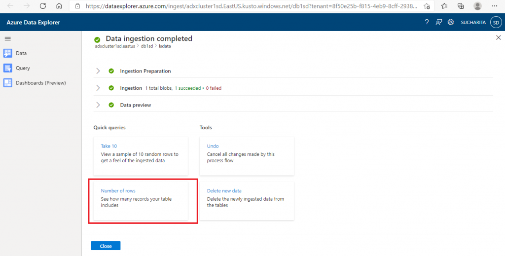
Once the data ingestion is completed, the data is ready for preview and querying. The ingestion steps and details are available here for reference. A few quick query options are available. I select and press the Number of rows query option.

Step 7: Show the query result

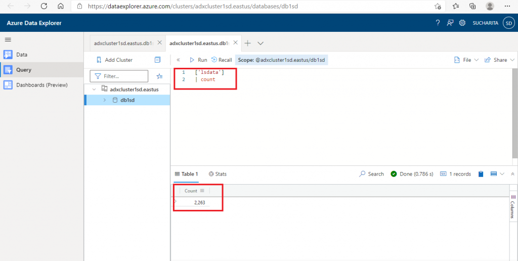
In the Query tab, the query and the result are shown for the number of rows in the lsdata table as created and populated in the earlier steps. This query language is known as Kusto Query Language (KQL). It is similar to SQL.

A Kusto query is a read-only request to process data and return results. This query consists of a sequence of query statements. These statements are delimited by semicolon. In every query, there should be at least one  tabular expression statement which returns data in a table-column format. KQL allows to send data queries and use control commands.

A query is a read-only request to process data, It returns the results of the processing, but does not modify the data or metadata. Control commands are requests to Kusto to process and potentially modify data or metadata.

Step 8: Query result visualization

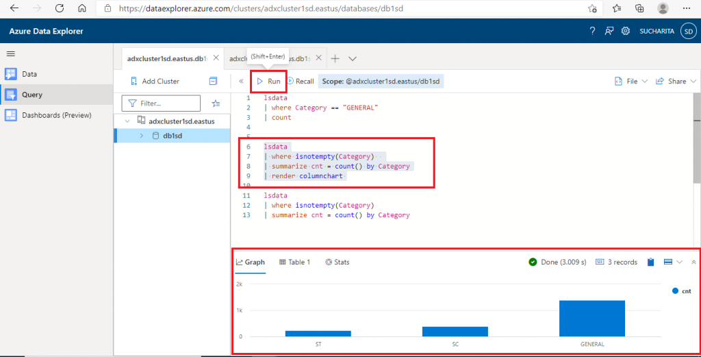
I write another KQL query to find the count of different values in the Category column. I eliminate the NULL values as well with the WHERE clause. In the last statement, I used render operation to visualize the query result graphically with a column chart.

After writing the query, I press the 'Run' button. The query output is generated at the bottom window. Apart from the graphical output, the tabular output is also generated. Performance details of the query is also available along with the query result. Also, it is possible to save and download the query output data in files.

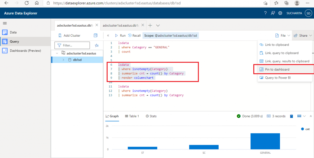
Step 9: Pin to Dashboard

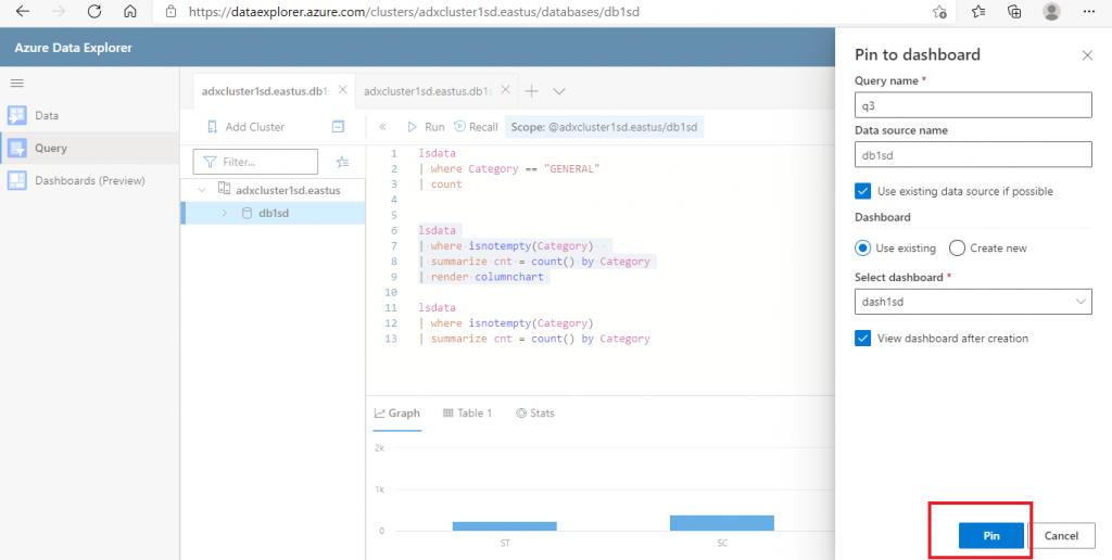
It is possible to share the query results in the ADX dashboard for reporting purposes. In the query window, there is an option to share the query result to the Dashboard. I select the query and press the 'Pin to Dashboard' option. A pop-up window opens where I need to supply the Query name and the Dashboard name. I may create a new dashboard or select an existing one. After providing the required details, I press the 'Pin' button.

The ADX Dashboard is a web application in Azure Data Explorer that helps to run queries and build dashboards. Data rendering performance from the ADX query is optimized.

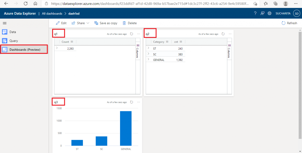
Step 10: Dashboard View

This is the Dashboards tab. Here, the output of the pinned queries are available together.

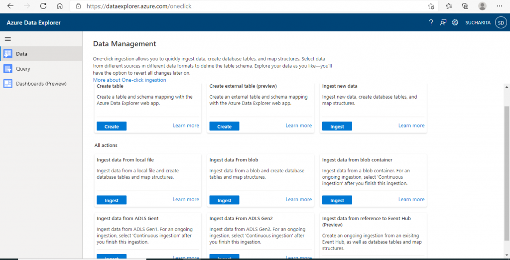
Step 11: Data View

I go to the Data tab. Here, I may continue with table creation and data ingestion. Various options are available for a these tasks.

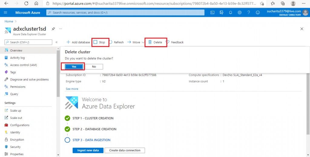
Step 12: Delete the cluster

I go back to the Overview tab of the ADX cluster, where I may stop the cluster when it is not in use. Then, it is possible to restart the cluster again. That will save the processing cost incurred when the cluster is not in use.

If I delete the cluster, everything related to the cluster will be deleted permanently.

Conclusion

In this article, I gave an overview of Azure Data Explorer. I explained the required steps for ingesting data from an input .csv file from my local drive and running query and visualizing the query results through ADX.

There are many different sources and types of data that can be ingested and processed through ADX. We need to decide on the values for cluster parameters based on the requirement. The best configurations also incur the maximum cost. When the cluster is not in use, it can be stopped for cost saving. For analyzing the data, it is required to be familiar with Kusto Query Language (KQL). I used a few basic KQL queries here. We may discuss in detail about each topic in separate articles.