Throughout this Stairway, we often state that a certain query executes in a certain way; and we cite the generated query plan to support our statement.  Management Studio’s display of estimated and actual query plans can help you determine the benefit, or lack thereof, of your indexes.  Thus, the purpose of this level is to give you sufficient understanding of query plans that you can:

• Verify our assertions as you read this Stairway.
• Determine if your indexes are benefiting your queries.

There are many articles on reading query plans, including several in the MSDN library. It is not our intention here to extend or replace them. In fact, we will provide links / references to many of them in this level. A good place to start is Displaying Graphical Execution Plans (http://msdn.microsoft.com/en-us/library/ms178071.aspx). Other useful resources include Grant Fritchey's book, SQL Server Execution Plans (available for free in eBook form), and Fabiano Amorim's series of Simple-Talk articles about the various operators found in your query plan output (http://www.simple-talk.com/author/fabiano-amorim/).

Graphical Query Plans

A query plan is the set of instructions that SQL Server follows to execute a query.  SQL Server Management Studio will display a query plan for you in text, graphical, or XML format.  For instance, consider the following simple query:

SELECT LastName, FirstName, MiddleName, Title 
FROM Person.Contact
WHERE Suffix = 'Jr.'
ORDER BY Title

The plan for this query could be viewed as shown in Figure 1.

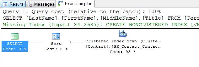
Figure 1 – Actual query plan in graphical format

Alternatively, it could be viewed as text:

|--Sort(ORDER BY:([AdventureWorks].[Person].[Contact].[Title] ASC))

|--Clustered Index

Scan(OBJECT:([AdventureWorks].[Person].[Contact].[PK_Contact_ContactID]),

WHERE:([AdventureWorks].[Person].[Contact].[Suffix]=N'Jr.'))

Or as an XML document, starting like this:

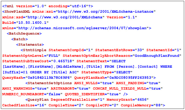
The display of query plans can be requested as follows:

• To request the graphical query plan, use Management Studio’s SQL Editor Toolbar, which has both a “Show Estimated Execution Plan” and an “Include Actual Execution Plan” button. The “Show Estimated Execution Plan” option displays the query plan graph for the selected TSQL code immediately, without executing the query. The “Include Actual Execution Plan” button is a switch, and once you have selected this option, every query batch that you execute will show you the query plan graph in a new tab, along with the results and the messages. This option can be seen in Figure 1.
• To request the text query plan, use the SET SHOWPLAN_TEXT ON statement.  Turning the text version on will turn the graphical version off and will not execute any of your queries.
• To view the XML version, right click within the graphical version and chose “Show Execution Plan XML” from the context menu.

For the remainder of this level, we focus on the graphical view, as it normally provides the fastest understanding of the plan.  For query plans, one picture is usually better than a thousand words.

Reading Graphical Query Plans

Graphical query plans are usually read from right to left; with the right most icon(s) representing the first step in a data gathering stream.  This is normally the accessing of a heap or index.  You will not see the word table used here; rather, you will see either clustered index scan or heap scan.  This is the first place to look to see which indexes, if any, are being used.

Each icon in a graphical query plan represents an operation.  For additional information on the possible icons, see Graphical Execution Plan Icons at http://msdn.microsoft.com/en-us/library/ms175913.aspx

The arrows that connect the operations represent the rows, streaming out of one operation and into the next.

Placing your mouse over on icon or arrow will cause additional information to be displayed.

Do not think of an operation as a step, for this implies that one operation must be completed before the next operation can begin.  This is not necessarily true.  For instance, when a WHERE clause is evaluated, that is, when a Filter operation is performed, rows are evaluated one at a time; not all at once.  A row can move to the next operation before a subsequent row arrives at the filter operation.  A Sort operation, on the other hand, must be completed in its entirety before the first row can move to the next operation.

Using Some Additional Information

A graphical query plan displays two pieces of potentially helpful information that are not part of the plan itself; suggested indexes and the relative cost of each operation.

In the example shown above, the suggested index, shown in green and truncated by space requirements, recommends a nonclustered index on Contact table’s Suffix column; with included columns of Title, FirstName, MiddleName, and LastName.

The relative cost of each operation for this plan informs us that the sort operation was 5% of the total cost, while the table scan was 95% of the work.  Thus, if we want to improve the performance of this query, we should address the table scan, not the sort; which is why an index was suggested. If we create the recommended index, like this:

CREATE NONCLUSTERED INDEX IX_Suffix ON Person.Contact
(
Suffix
)
INCLUDE ( Title, FirstName, MiddleName, LastName )

And then rerun the query, our reads drop from 569 to 3; and the new query plan, shown below, shows why.

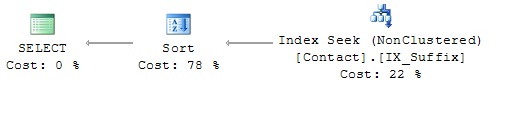
The new nonclustered index, with its index key of Suffix, has the “WHERE Suffix = 'Jr.'“ entries clustered together; hence, the reduction in IO required to retrieve the data.  As a consequence, the sort operation, which is the same sort operation that it was in the previous plan, now represents over 75% of the total cost of the query, instead of the mere 5% of the cost that it had been.  Thus the original plan required 75 / 5 = 15 times the amount of work to gather the same information as the current plan.

Since our WHERE clause includes only an equality operator, we can improve our index even more by moving the Title column into the index key, like so:

IF  EXISTS (SELECT * FROM sys.indexes
WHERE OBJECT_ID = OBJECT_ID(N'Person.Contact')
AND name = N'IX_Suffix')
DROP INDEX IX_Suffix ON Person.Contact
CREATE NONCLUSTERED INDEX IX_Suffix ON Person.Contact
(
Suffix, Title
)
INCLUDE ( FirstName, MiddleName, LastName )

Now, the needed entries are still clustered together within the index, and within each cluster they are in the requested sequence; as indicated by the new query plan, shown in Figure 2.

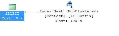
Figure 2- Query Plan after rebuilding the nonclustered index

The plan now shows that the sort operation is no longer needed. At this point, we can drop our highly beneficial covering index.  This restores the Contact table to the way it was when we started; which is the state we want it to be in as we enter our next topic.

Viewing Parallel Streams

If two streams of rows can be processed in parallel, they will appear above and below each other in the graphical display.  The relative width of the arrows indicates how many rows are being processed through each stream.

For instance, the following join, extends the previous query to include sales information:

SELECT C.LastName, C.FirstName, C.MiddleName, C.Title
, H.SalesOrderID, H.OrderDate
FROM Person.Contact C
JOIN Sales.SalesOrderHeader H ON H.ContactID = C.ContactID
WHERE Suffix = 'Jr.'
ORDER BY Title

The query plan is shown in Figure 3.

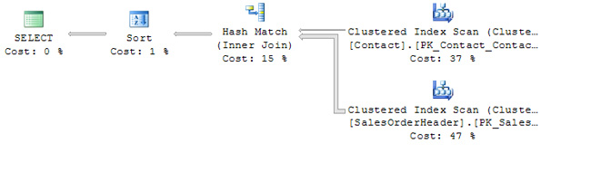
Figure 3 – A query plan for a JOIN

A quick look at the plan tells us a few things:

• Both tables are scanned at the same time.
• Most of the work is spent in scanning the tables.
• More rows come out or the SalesOrderHeader table than out of the Contact table.
• The two tables are not clustered into the same sequence; therefore matching each SalesOrderHeader rows with its Contact row will require extra effort.  In this case, a Hash Match operation is used.  (More on hashing later.)
• The effort required to sort the selected rows is negligible.

Even individual streams of rows can be broken into separate streams of fewer rows each to take advantage of parallel processing.  For example, if we change the WHERE clause in the above query to WHERE Suffix is NULL.

Far more rows will be returned, as more the 95% of the Contact rows have a NULL Suffix.  The new query plan reflects this, as show in Figure 4.

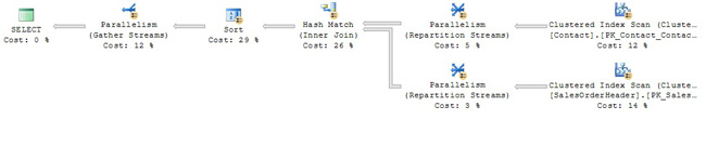
Figure 4 – A parallel query plan

The new plan also shows us that the increased number of Contact rows has caused the Match and Sort operations to become the critical path for this query.  If we need to improve its performance, we must attack these two operations first.  Once again, an index with included columns will help.

Like most joins, our example joins two tables via the foreign key / primary key relationship.  One of those tables, Contact, is sequenced by ContactID, which also happens to be its primary key.  In the other table, SaleOrderHeader, ContactID is a foreign key.  Since ContactID is a foreign key, requests for SaleOrderHeader data accessed by ContactID, such as our join example, might be a common business requirement.  These requests would benefit from an index on ContactID.

Whenever you are indexing a foreign key column, always ask yourself what, if any, columns should be added, as included columns, to the index.  In our case, we have just one query rather than a family of queries to support.  Thus, our only included column will be OrderDate.  To support a family of ContactID oriented queries against the SaleOrderHeader table, we would include more SaleOrderHeader columns in the index, as needed, to support those additional queries.

Our CREATE INDEX statement is:

CREATE NONCLUSTERED INDEX IX_ContactID ON Sales.SalesOrderHeader
(
ContactID
)
INCLUDE ( OrderDate )

And the new plan for executing our join of SalesOrderHeader and Contact information is in Figure 5.

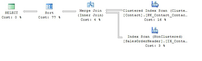
Figure 5 – Plan for a JOIN query with a supporting index on each table

Because both input streams now are sequenced by the join predicate column, ContactID; the JOIN portion of the query can be done without splitting the streams and without hashing; thus reducing what was 26 + 5 + 3 = 34% of the work load down to 4% of the work load.

Sorting, Presorting and Hashing

Many query operations require that data be grouped before the operation can be performed.  These include DISTINCT, UNION (which implies distinct), GROUP BY (and its various aggregate functions), and JOIN.  Normally, SQL Server will use one of three methods to achieve this grouping, the first of which requires your assistance:

• Happily discover that the data has been presorted into the grouping sequence.
• Group the data by performing a hashing operation.
• Sort the data into the grouping sequence.

Presorting

Indexes are your way of presorting data; that is, of providing data to SQL Server in frequently needed sequences.  This is why the creation of nonclustered indexes, each containing included columns, benefited our previous examples.  In fact, if you place your mouse over the Merge Join icon in the most recent query, the phrase Match rows from two suitably sorted input streams, exploiting their sort order. will appear.  This informs you that the rows of the two tables / indexes were joined using the absolute minimum of memory and processor time.  Suitably sorted input is a wonderful phrase to see when mousing over query plan icons, for it validates your choice of indexes.

Hashing

If the incoming data is not in a desirable sequence, SQL Server may use a hashing operation to group the data.  Hashing is a technique that can use a significant amount of memory, but is often more efficient than sorting.  When performing DISTINCT, UNION, and JOIN operations, hashing has an advantage over sorting in that individual rows can be passed to the next operation without having to wait for all incoming rows to be hashed.  When calculating grouped aggregates, however, all input rows must be read before any aggregate values can be passed to the next operation.

The amount of memory required to hash information is directly related to the number of groups required.  Thus the hashing required to resolve:

SELECT Gender, COUNT(*)
FROM NewYorkCityCensus
GROUP BY Gender

Would require very little memory, for there would be only two groups; Female and Male, regardless of the number of input rows. On the other hand:

SELECT LastName, FirstName, COUNT(*)
FROM NewYorkCityCensus
GROUP BY LastName, FirstName

Would result in an enormous number of groups, each requiring its own space in memory; possibly consuming so much memory that hashing becomes an undesirable technique for resolving the query.

For more on query plan hashing, visit http://msdn.microsoft.com/en-us/library/ms189582.aspx.

Sorting

If the data has not been presorted (indexed) and if SQL Server deems that hashing cannot be done efficiently, SQL Server will sort the data.  This is normally the least desirable option.  Therefore, if a Sort icon appears early in the plan, check to see if you can improve your indexing.  If the Sorticon appears near the end of the plan, it probably means that SQL Server is sorting the final output into the sequence requested by an ORDER BY clause; and that this sequence differs from the sequence that was used to resolve the query’s JOINs, GROUP BYs, and UNIONs. Usually, there is little you can do to avoid the sort at this point.

Conclusion

A query plan shows you the methodology SQL Server intends to use, or has used, to execute a query.  It does so by detailing the operations that will be used, the flow of the rows from operation to operation, and the parallelism involved.

• You view this information as a text, graphical, or XML display.
• Graphical plans show the relative work load of each operation.
• Graphical plans may suggest an index that will improve the performance of the query.
• Understanding query plans will help you evaluate and optimize your index design.