In Level 10, while explaining why an index needed a non-leaf portion as well as a leaf portion, we said: “SQL Server, however, has no intrinsic knowledge of English language last names, or of any other data.” Thus, SQL Server does not know whether the “Meyer, Helen” entries represent 50 percent, or .05 percent of the entries in the index.

But it needs to know something about your data’s distribution; because, as we have seen, the selectivity of the query is a major factor in deciding whether an index should be used or not. Therefore, for every index, SQL Server maintains a small amount of information about the data values contained in the index key columns. This information is called index statistics, or sometimes just statistics, and it is the subject of this Level.

Statistics can also be generated for columns that do not appear in an index. The structure of those statistics is identical to index statistics. Since this Stairway is about indexes, all discussion will refer to index statistics.

Index statistics are a bit like the engine in your car: It is nice to know how it works internally, but more important is scheduling regular preventive maintenance with someone who does know how an engine works. We will cover both aspects if index statistics in this Level; describing the internals of index statistics and explaining when and why your statistics will need maintenance.

The Structure of Index Statistics

Index statistics are divided into three parts; the header, density vector, and histogram. To view the complete statistics for an index, you can execute:

DBCC SHOW_STATISTICS (tablename, indexname)

To view each part individually, execute:

DBCC SHOW_STATISTICS (tablename, indexname) WITH STAT_HEADER

Or:

DBCC SHOW_STATISTICS (tablename, indexname) WITH DENSITY_VECTOR

Or:

DBCC SHOW_STATISTICS (tablename, indexname) WITH HISTOGRAM

But, before we can view statistics, we need a table and an index to use as an example. Our sample table will consist of three columns and two indexes; one index on the first two columns, and one on the third column; as shown in Listing 1.

Listing 1: A Sample Table with Two Indexes

We also need some sample data; data with specific patterns to help illustrate index statistics. We generate 5050 rows of this sample data with the code shown in Listing 2.

Listing 2: The Sample Data Generator

The resulting sample data will have the following characteristics:

Each value that appears in Col1 will appear in as many rows as the value. Thus, 1 will appear in one row, 2 will appear in two rows; 3 will appear in three rows, and so on.

For any row, the combination of the Col1 - Col2 values is unique within the table. That is, IX_HistogramTest could have been specified as a unique index.

The values appearing in Col3 are also unique, starting at 1 and incrementing by 1 for each row thereafter. Thus, IX_SingleValue also could have been a unique index.

For demonstration purposes, we create the table but not the indexes; load the table; then create the indexes. This gives the best load performance and ensures that our index statistics are up-to-date.

Once we have loaded the table and created the indexes, we run the queryshown in Listing 3, to verify that our sample data has the characteristics mentioned above. The results, shown in Figure 1, verify that our data has the specified three characteristics.

And, because the results shown in Figure 1 are in Col1 - Col2 sequence, Figure 1, minus Col3, also represents a sample portion of the IX_HistogramTest index.

Listing 3: Query the Sample Data

Figure 1: A subset of our sample data

Density

One common term that you encounter when dealing with statistics is density. Density is a measure of uniqueness of values, and is directly related to selectivity; a term that we have used in earlier levels. For example, an index key density of 0.01 means that are 1 / 0.01 = 100 different values in the index key. To put it another way; each value occurs, on average, in 1 out of every 100 entries. Density can be measured on individual columns or on a composite of columns, such as Col1 – Col2.

If Figure 1 were the entire table, rather than a subset of the rows, the density of Col1 would be 1 / 6 = 0.1667; while the density of Col3 would be 1 / 20 = 0.05.

The smaller the density, the fewer the rows that will match an equality comparison, and the more selective a WHERE clause such as WHERE Col3 = 17 will be.

The Statistics Header

When we execute:

We receive the index statistics header shown in Figure 2.

Figure 2: The Index Statistics Header

The header’s fields tell us the following:

Name: The name of the index is IX_HistogramTest.

Updated: The statistics were last updated April 18th at 2:16pm. (In our case, they were initially generated at that time; they have never been updated.)

Rows: The number of entries in the index is 5050. This number is always the number of entries in the index, not the number of rows in the table. See the Unfiltered Rows definition below.

Rows Sampled: The number of entries that were sampled to generate these statistics is 5050. (More on sampling later.)

Steps: The number of steps in the histogram portion of the statistics is 59. (More on steps later.)

Density: This value is not used by SQL Server 2008 and exists solely for backward compatability.

Average Key Length: The average length of the index key values is 8. In our case, all the keys are fixed width of size 8 bytes; consisting of two 4 byte integers, Col1 and Col2.

String Index: These statistics do not include string summary statistics. (More on string summary statistics later.)

Filter Expression: This index was not created with a FILTER clause specified.

Unfiltered Rows: The number of rows in the underlying table is 5050. If this were a filtered index, this number could be greater than the Rows value.

The Statistics Density Vector

When we execute:

We receive the index density vector shown in Figure 3.

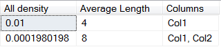
Figure 3: The Index Statistics Density Vector

The density vector values shown in Figure 3 tell us:

Col1 averages 4 bytes in size, and contains 1 / 0.01 = 100 distinct values; the number that we would expect, given the sample data generation code shown in Listing 2.

The composite of Col1 - Col2 is 8 bytes in size and contains 1 / 0.0001980198 = 5050 distinct values; also a number that we expect, for we said earlier that this value would be unique across the index.

The Statistics Histogram

When we execute:

We receive an index histogram; whose first 25 steps, out of 59, are shown in Figure 4.

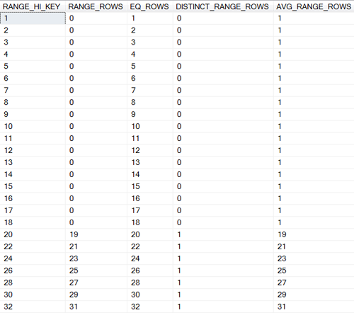
Figure 4: The first 25 steps of our Index Statistics Histogram

The histogram looks like a table with five columns. However, the correct term for each item is step, not row. All the values in a histogram are derived from values the left most column of the index key. In the case of IX_HistogramTest, this column is Col1. All other columns are ignored in the generation of a histogram.

Each step of a histogram spans, or represents, a consecutive set (a range) of the index’s entries. A histogram will never have more than 200 steps; regardless of the size of the table. Different steps may span a different number of entries; perhaps with one step being derived from 30 entries and the next step representing the next 46 entries.

To help explain the individual values of a histogram, we define the following four terms here; and illustrate them in Figure 5:

The left value of an index entry is the value contained in the entry’s left most column. Thus, in our sample, this is the value of Col1.

A step set is the set of consecutive index entries represented by a step. All the values in a step’s five columns are derived from the left values contained in the step’s step set.

The upper subset of a step set is those entries whose left value is equal to the highest left value found in the step set.

The lower subset of a step set is those entries whose left value is less than the highest left value found in the step set.

For example, the index step set shown in Figure 5 generated the Figure 4 step whose RANGE-HI-KEY value is 20.

Figure 5: A Step Set within an Index

Because this, our first sample, has only 100 different left values, each step spans two or less left values. Later in this Level, when we increase the sample’s row count by a multiple of 100, we will see steps that span a much large range of left values.

The values in the five columns of a histogram, such as the one shown in Figure 4, are calculated as follows:

Note: Since the first and third columns of the histogram are derived from the step’s upper subset, we define them first. The remaining three columns, derived from the step’s lower subset, are defined last.

RANGE_HI_KEY:

The highest left value in the step’s step set. The RANGE_HI_KEY value identifies the step; thus, two steps will never have the same RANGE_HI_KEY value.

For the first step, RANGE_HI_KEY is the lowest left value in the index. Thus, the first step always has an empty lower subset. For the last step, RANGE_HI_KEY is the highest left value in the index.

Steps are maintained, and displayed, in RANGE_HI_KEY sequence.

In our example, the first step has a RANGE_HI_KEY value of 1, which is the lowest Col1 value in the index; the last step has a RANGE_HI_KEY value of 100, which is the highest Col1 value in the index. None of the 59 steps have the same RANGE_HI_KEY RANGE_HI_KEY value.

Since the RANGE_HI_KEY value identifies a step, a step is referred to by that value. Thus, the step whose RANGE_HI_KEY = 20, is known as Step 20; regardless of whether it is the 3rd step or the 33rd step in the histogram.

EQ_ROWS:

The number of entries whose left value equals RANGE_HI_KEY; that is, the number of entries in the step’s upper subset.

In our example, Step 20 tells us that there are 20 entries in the index with a left value of 20; something we already knew from the algorithm we used to generate our sample data.

RANGE_ROWS:

The number of entries in the step’s lower subset. RANGE_ROWS will always be 0 for the first step.

In our example, Step 20 tells us that there are 19 entries with a left value between 18 and 20. We know this value is correct because we generated our sample data to have 19 rows with a left value of 19, and because 19 is the only left value that lies between 18 and 20.

DISTINCT_RANGE_ROWS:

The number of distinct left values in the step’s lower subset.

In our example, Step 20 tells us that the 19 entries with a left value between 18 and 20 have only 1 distinct value; that is, they all have the same value. Again, this is a consequence of our data generating algorithm.

AVG_RANGE_ROWS:

The average number of rows per distinct left value in the step’s lower subset; specifically, RANGE_ROWS / DISTINCT_RANGE_ROWS. If RANGE_ROWS is 0, this number is 1; more correctly, if RANGE_ROWS is 0, this number is meaningless.

Examining a Large Sample

Our previous example was relatively small; it was so small that we could easily verify the values that appeared in our statistics. But small tables are not the ones that need statistics. It is in the querying of large tables that SQL Server must make the best decision regarding which indexes to use, or suffer the performance conseuences. For this reason, we increase the row count of our sample table.

In short, we change the first DECLARE of our sample data generating code shown in Figure 2 from:

To:

Then we recreate the table, reload the data, and recreate the indexes. This gives us a table of 500,500 rows. The highest Col1 value in the table is 1000; a value that appears in 1000 rows.

When we execute:

We receive the index statistics shown in Figure 6; minus the last 194 steps, which we truncated for the sake of brevity.

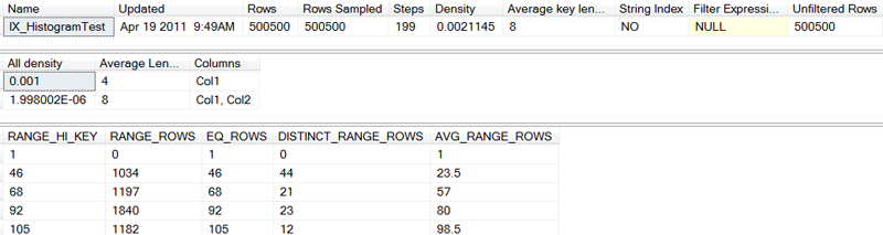
Figure 6: Index Statistics for a Large Example

The second step, with a left value of 46, indicates that its upper sub set contains 46 rows (each with a left value of 46), which concurs with our data loading algorithm. Also concurring with our data loading algorithm is the step’s specification that there are 1034 (2 + 3 + 4 … + 44 + 45) rows in the step’s lower subset, and that those rows contain 44 different left values (2 through 45); yielding an average of 23.5 rows per left value.

Thus, if SQL Server is resolving:

…it will expect 46 of the 500,500 rows to meet that criteria.

If the clause were:

…it would expect 23.5 of the 500,500 rows to meet the criteria.

Even a less precise clause like:

…would still enable SQL Server to anticipate that 517 rows (one half of all the rows in the lower subset) will be selected.

Unique Indexes and Statistics

Both our indexes, IX_HistogramTest and IX_SingleValue, could have been created as UNIQUE indexes; and in a real world scenario they should have been. Index statistics can indicate that the values in the index probably are unique, but they can never guarantee it; and index statistics will never cause SQL Server to enforce uniqueness of values within the index. In Level 8 – Unique Indexes, we saw how the designation of an index as UNIQUE caused SQL Server to choose a better execution plan; something that statistics alone would not have caused.

Conversely, just knowing that an index’s values are unique does not give SQL Server any idea of what those values are. To know the range of values in our IX_SingleValue index, the one that has the characteristics of a single-column primary key index, SQL Server must examine its statistics. For us, that means executing:

…and examining the results shown in Figure 7.

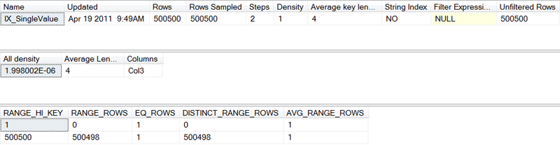
Figure 7: Index statistics for a single-column unique index

Note that it only takes two steps to tell SQL Server all that it needs to know:

The index contains 500500 entries.

Those entries contain 500500 (1 + 500548 + 1) different values, ranging from 1 through 500500.

Regardless of whether a future WHERE clause that references Col3 contains an =, or >, or < or a BETWEEN; SQL Server can quickly and accurately estimate the number of rows that it will return.

String Summary Statistics

Strings (char, varchar, text, nchar, nvarchar, and ntext) are different from numeric data types in that they are not truly atomic. Functions like substring and operators like LIKE can cause SQL Server to examine a subset of the characters in a string value. For this reason, there is a need for statistics that will help SQL Server make decisions regarding the probability of certain substrings occurring with values of a string column. These statistics are called String Summary Statistics, and they are new to SQL Server 2008.

If the statistics header’s StringIndex column has a value of ‘YES’, then SQL Server has generated string summary statistics for the left most column of the index key. If the left most column of the index contains string values that are greater than 80 characters long, only the first 40 and the last 40 characters will be used to generate the string summary statistics.

Executing DBCC SHOW_STATISTICS does not display the string summary statistics; nor does any other supported T-SQL command.

Maintaining Index Statistics

All this index statistics capability that we have just seen is very nice; but it is of no benefit if the statistics are not up-to-date. More correctly, it is of no benefit if the values in the statistics do not reflect the values in the index. And statistics can become out-of-date because SQL Server does not update statistics every time data in the table is modified causing an entry to be added to or deleted from an index. In a sense, SQL Server never updates statistics, it only regenerates them. (We use both terms interchangeably in this Level.) And regenerating statistics is an effort that we do not want SQL Server to do more often than necessarily.

Therefore, we need to look at controlling the effort required to update statistics and at when to update statistics.

When to Update Index Statistics

Fortunately, SQL Server gives you control over when index statistics are regenerated.

Every database contains an AUTO_UPDATE_STATISTICS option. By default this option ON when the database is created, and can be toggled by the ALTER DATABASE command. When this option is ON, SQL Server will regenerate statistics for an index after a preset number of data modifications against the table have occurred. The number of data modifications required before statistics are updated is determined by SQL Server; it is based on the number of rows in the table; and is not configurable.

When you create or alter an index, you can use the STATISTICS_NORECOMPUTE option of the CREATE INDEX statement to specify whether the index’s statistics should be automatically updated or not.

If you wish to explicitly regenerate index statistics at any time, you can execute:

UPDATE STATISTICS SchemaName.TableName

The above command will regenerate statistics on all indexes of the specified table. Or you can execute:

UPDATE STATISTICS SchemaName.TableName IndexName

The above command will regenerate statistics for the specified index.

In addition, the stored procedure sp_updatestats can be used to have statistics regenerated for every index on every table in the entire database.

In general, AUTO_UPDATE_STATISTICS is best. It relieves you of an administrative burden and it normally results in good statistics generation with minimal impact on other processes.

Some reasons for wanting to override this default option, and control the generation of statistics yourself are:

You have a regular predefined maintenance window, and wish to update statistics at that time.

The table is too large; the updating of statistics would take too long to allow it to be done automatically; manual updating at a specified time would be better.

The index has many unique index key values. This requires a large sample to obtain meaningful statistics. The default sample percentage is not large enough to provide this reliability.

Changes to the table cause the statistics to become unreliable faster than SQL Server expects.

To illustrate this last condition, and to understand why you might want to override the auto update option, consider the following table, whose creation script is shown in Listing 4. It is a table used by a large lending library to track books that are currently loaned out to its members.

Listing 4: The Loan table

Each time a book is loaned, a row is added to the table. When the book is returned, that row is removed.

For each loan, four pieces of information are recorded:

The member number of the member who borrowed the book.

The ISBN (International Standard Book Number) of the book that was borrowed.

The date that the book was borrowed.

The date that the book is due.

Since most borrowers adhere to the requirement that a borrowed book be returned in fourteen days, there is a near 100% turnover of rows in the table every two weeks; every returned book results in a row being deleted; every loan results in a row being inserted. During that two week period, the distribution of values in the ISBN column remains almost unchanged; while the distribution of values in the DueDate column completely changes.

There is nothing about a book’s ISBN that would make it popular this month and unpopular next month. Thus, the distribution of values in the ISBN column will be the same this month as last month. Many of the individual ISBN numbers will be different, but the range of values remains the same.

This is not true for the DueDate column. This month, the due date values range from today to today + fourteen days. One month from now, they will range from today + one month to today + one month + fourteen days. There is no overlap in those two ranges. If the statistics are not updated during this period of time, no DueDate histogram step will represent values that are actually in the index.

Thus, DueDate index statistics need to be updated more frequently than ISBN index statistics.

Minimizing the Impact of Update Statistics

SQL Server also gives you control over how much of the index must be read when updating the index’s statistics.

When an index is created, all the index entries must be processed. Therefore, all the entries participate in calculating the index’s statistics.

But when statistics are subsequently updated, accessing all the entries is normally overkill. For a large index, accessing the entire leaf level requires considerable IO; while a much smaller sampling of the leaf level entries normally suffices. Therefore, whenever SQL Server updates index statistics, by default, it takes a sampling of the entries in the index.

SQL Server determines the sample size, but you can override it. Whenever you explicitly update index statistics, you can specify the SAMPLE n PERCENT, or the SAMPLE n ROWS, or the FULLSCAN option. Whatever value you specify with the PERCENT or ROWS option will be used for that statistics update and will remain in effect for subsequent automatic updates.

To illustrate that sampling, not full scan, is the default for regenerating statistics, we reload our sample table with the same 500,500 rows that we used in the last example. Only this time, immediately after creating the indexes, we execute:

Now, when we execute:

We receive the results shown in Figure 8, not the results shown in Figure 6.

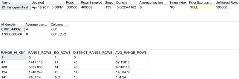
Figure 8: Index Statistics from a Sampling

Although the statistics shown in Figure 8 are similar to those of Figure 6, they are not identical. In the histogram, precise data values in the RANGE_ROWS column have been replaced with floating point estimations. The sample was large, approximately 80% of the rows, but it was still a sample.

Summary

Index statistics help SQL Server optimize queries.

Index statistics are generated whenever an index is created or rebuilt.

Index statistics are divided into three parts, and can be viewed by executing:

Index statistics can become out-of-date. If they do, they can result in poor decisions by the query optimizer.

By default, index statistics are regenerated automatically. You can turn off this automatic regeneration. You can also force a manual regeneration of statistics for an index or for a table.

Regenerating index statistics is normally done by sampling the index, rather than by reading the entire leaf level of the index. You can control the size of the sample that is used to regenerate an index’s statistics.