

By Steve Bolton
…………One of the major thrusts of my various mistutorial series has been to drive home the point that SQL Server’s set-based languages can be efficiently applied to a wider variety of data mining tasks than is generally appreciated. In some instances a well-indexed and coded stored procedure can perform much better than the graphics card-based processing that is now the rage among certain applications; these are a sound choice for calculations heavy in matrix math and low in precision, but lack the flexibility that set-based logic provides and sometimes also lag in terms of performance. R has been widely adopted in the data science community, but has some insurmountable limitations when it comes to handling the large recordsets that SQL Server relational databases and Analysis Services are adept at handling; on the other hand, R and competitors like WEKA and Minitab are often a better choice for ordinary lower-level statistical tests, particularly on smaller tables. Most of the measures of information I’ve discussed so far in this series can be calculated quite efficiently on very large recordsets, but I’d be negligent if I did not at least mention one glaring exception: Fisher Information, particularly in its matrix form. The good news is that its major use case is not one we’re likely to encounter much in the realm of relational databases, where record counts in the thousands and millions are routine and sometimes even surpass the billion-row mark in “Big Data” applications.
…………The relative unsuitability of the Fisher Information Matrix is best revealed by walking through the lengthy process of its derivation, which will involve at least a cursory explanation at each step. Along the way we will encounter some of the common nemeses of relational database mining, like matrix math, derivatives, integrals and algebraic manipulation, all of which we’re better off calculating with other tools like those mentioned above. Derivatives and integrals are normally calculated through algebraic manipultation upon well-defined functions in the mathematical literature, to the point that it is exceedingly difficult to locate algorithms for estimating them from data in reverse. I nevertheless managed to cobble together two interlocking T-SQL stored procedures awhile back for estimating derivatives, after gleaning the general workflow from this website and informal tutorial, both which are now defunct. The corresponding procedure for estimating integrals was sittched together from the Wikipedia article on Riemann Sums and an online course book on calculus.[ii] It too requires more thorough testing, but is at least noticeably less complicated. The same cannot be said for the series of fifteen interlocking functions needed to calculate matrix inverses in T-SQL, a structure I’ve gradually refined in the course of occasional experimentation. This does not include two others needed to accommodate primary keys, two others for traces and eigenvalues, three stored procedures for calculating covariance, inverse covariance and correlation matrices and several calling stored procedures to instantiate the required temp tables.
…………This monstrous complexity could be significantly reduced if not for a whole obstacle course of artificial T-SQL limitations that Microsoft could conceivably remove, like the fact that LEAD and LAG won’t update correctly inside a recursive CTE and prohibition against updating values within functions; among the silliest is the non-updatability of table-valued parameters, which mandates extra code to recreate each TVP passed to these procedures and cache the data within them, all of which adds to the performance costs. We are also prevented from returning a TVP from a stored procedure for some reason. The structure described above performs reasonably well despite the complexity imposed by such constraints, but still runs into a brick wall in the form of the “No more lock classes available” error when the recursion required to calculate matrix determinants surpasses Microsoft’s recursion nesting limit of 32. SQL Server wasn’t designed with matrices in mind but can be cajoled into calculating determinants and inverses of fairly small ones with a fair level of success, one that could probably be improved with adjustments to these constraints on Microsoft’s part.
…………Pushing the boundaries of SQL Server can be commendable, but one thing we can’t do at all is solve algebraic equations, at least not without comical clumsiness. I usually post sample code in my data mining articles, but there is no point in setting a Guinness record for the longest sequence of T-SQL code just to accommodate the matrix procedures alone, when we would also have to incorporate derivative, integral and algebraic routines as well in order to derive the Fisher Information Matrix. The simultaneous presence of all of these stumbling blocks is a strong clue this particular data mining task could be better solved by tools designed with these uses in mind. This is doubly true when we consider just what Fisher Information is designed to measure – which is thankfully probably already available to us almost free of charge, thanks to the relatively high record counts we’re accustomed to.
Minimizing the Costs of Maximum Likelihood Estimation
It’s quite difficult to find an intuitive explanation of Maximum Likelihood Estimation (MLE), let alone the Fisher Information derived for it; there are exceptions, but many mathematicians reply to requests for explanations in layman’s terms for any topic with a flurry of equations, which are antithesis of intuitiveness to all but initiates in the arcane art of math, i.e. the “poetry of logic.” Don’t let the long name fool you though: MLE is a principle we all apply on a daily basis. As Chris Alvino, a machine learning expert at Netflix, points out, “every time you compute the mean of something, you’re effectively using maximum likelihood estimation. In effect, you’re making the assumption that the individual (real number) data points are independent draws from (the same) Gaussian with mean µ and some variance.”[iii] If you make an educated guess about the average value of something from a sample – such as the number of black T-shirts left in your closet based on the number in the hamper – then you’re applying the MLE principle at a beginner’s level. This is easiest to do with the normal or “Gaussian” distribution, i.e. the bell curve, since the variance and means of any sufficiently large sample we take will be commensurate to those of the actual population. In many cases the uncertainty of these “point estimates” serendipitously declines more rapidly than one might expect as the number of rows (or trials, in the case of experiments) rises, thereby capping the need for more data. Point estimates of the overall population can also be made for other statistics like counts or skewness, or on other distributions as long as they have an associated likelihood function. For the Bernoulli distribution, we might estimate the mean of a count of coin flips; for the Laplacian distribution, we’d be more apt to estimate the median.[iv] MLE can also be performed on regression equations[v] to determine the slopes, intercepts and error range, provided that we can calculate the statistical likelihood of their occurrence. We must also assume that the errors are independent and identically distributed (i.i.d.).
Figure 1: The PDF and Likelihood Functions of the Normal Distribution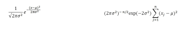
…………This is the first of many prerequisites, however, that rapidly complicate this relatively simple principle. First, we must make an educated guess about the function that produced the data, then derive a likelihood function from it, then estimate the statistics we need to plug into that likelihood function[vi], which is why the exercise is referred to as “parameter estimation.” As statistician Othman Nejjar puts it, “The likelihood function is nothing but the probability of observing this data given the parameters,”[vii] but determining this probability is no mean feat; in many cases this involves inverting the probability density function (PDF)[viii], involving a lot of algebra if one does not have a handy reference for that particular distribution’s likelihood function. What we’re essentially trying to do is determine the underlying data generation process (DGP) that produced our data, but without sufficient knowledge of the statistics. Data scientist Kingshuk Chatterjee provides the most intuitive explanation I’ve seen to date of what we’re seeking with MLE:
“The way I understand MLE is this: You only get to see what the nature wants you to see. Things you see are facts. These facts have an underlying process that generated it. These process are hidden, unknown, needs to be discovered. Then the question is: Given the observed fact, what is the likelihood that process P1 generated it? What is the likelihood that process P2 generated it? And so on… One of these likelihoods is going to be max of all. MLE is a function that extracts that max likelihood.”
…………“Think of a coin toss; coin is biased. No one knows the degree of bias. It could range from 0 (all tails) to 1 (all heads). A fair coin will be 0.5 (head/tail equally likely). When you do 10 tosses, and you observe 7 Heads, then the MLE is that degree of bias which is more likely to produce the observed fact of 7 heads in 10 tosses.”
…………“Think of a stock price of say, British Petroleum. BP was selling at $59.88 on April 23, 2010. By June 25, 2010 the price was down to $27.02. There could be several reasons for this fall. But the most likely reason could be the BP oil spill and the public sentiment. Stock price is the observed fact. The MLE will estimate the most likely underlying reason.”[ix]
…………This is akin to the goal of the procedures discussed in my series Goodness-of-Fit Testing with SQL Server, except with the focus on the inverses of the PDFs, rather than the cumulative distribution functions (CDFs), empirical distribution functions (EDFs) or PDFs used in those tests. We also have the added burden of having to estimate the statistics plugged in to the likelihood (or often log-likelihoods, which are sometimes more tractable) functions. A chicken-and-egg problem afflicts both goodness-of-fit testing and the subject of another mistutorial series of mine, Outlier Detection with SQL Server: do records fail to fit a distribution because the distribution itself is a poor fit, or are they merely outliers? With MLE, we still face the initial difficulty of selecting a distribution that reflects the underlying DGP, except now with a third consideration in the form of parameter estimation. That begs the question: why bother estimating these summary statistics anyways, if we can already calculate them with ease on large recordsets?
The Cramér–Rao Bound in the Era of Big Data
This is where Fisher Information comes in handy, because it can tell us just how many records we’d need to reduce the uncertainty of our parameter estimates to some subjectively predetermined level. What we seek is an estimation method that will yield statistics with a property known as “sufficiency,” [x] which means that we can’t learn anything more about a distribution by adding further samples than we already know from these numbers; various mathematical proofs (which I almost always omit in these articles) demonstrate that Fisher Information Metric “is the only Riemannian metric….that is invariant under sufficient statistics.”[xi] It is also possible to determine ahead of time in some cases the degree of error a particular method of estimation is prone to, which explains the derivation of the common terms “unbiased” and “biased estimator.”[xii] The faster the sufficiency of a statistic increases in tandem with the record count, the less biased the estimate will be; some increase linearly, others quadratically, all of which can be calculated beforehand in some cases. Others asymptotically approach (i.e. converge gradually as we approach infinity) what is known as the Cramér–Rao Bound[xiii], a mathematical lower limit on the variance of an unbiased estimator under certain preconditions.[xiv] This is determined by simply inverting the Fisher Information. Our estimate might perform worse than this, but we can at least move the boundary in the right direction by a predetermined distance by adding more records to our sample[xv], assuming they’re available to us. The aim is complementary to that for the well-known procedures for selecting sample sizes that yield predetermined confidence intervals for various statistical tests.[xvi] We can also apply various formulas to derive confidence intervals for our parameter estimates.[xvii]
…………One of the reasons I’ve usually omitted confidence intervals from my data mining self-tutorials is that these are calculated much more efficiently in ordinary statistical software, whether it be Excel, Minitab, R or one of their many competitors. The fact that we’re aiming at an analogous end ought to raise another red flag, which like the algebra involved in some likelihood function derivation, tells us that we’re moving out of the realm of justifiable SQL Server use cases. A more interesting question is whether or not the size of the data we typically deal with also renders the whole exercise moot, given that we often work with tables of thousands or millions of records, even billions in the case of Big Data. It may be a buzz word, but as I’ve pointed out before, many of the oldest statistical tests were designed for recordsets of just a few dozen rows, in ages when data of any kind was much harder to come by. A case in point is the Shapiro-Wilk goodness-of-fit test I expounded on long ago, which was originally limited to just 50 records and has recently been revised to accommodate up to 2,000, i.e. still a drop in the bucket compared to today’s huge tables. Even with what would now be considered small data, we’ve still long since passed the point where a small record count is going to impact the results much. Fisher Information was developed at the turn of the century – not our century, but the one before it, when pioneering statistician Ronald Fisher[xviii] was trying to squeeze as much information as he could out of quite small agricultural recordsets. Even in the present, the tutorials I’ve seen on Fisher Information envision recordsets of just a few hundred in their hypothetical examples. It’s quite likely in many of our use cases that the aggregates we calculate on our SQL Server tables are already sufficient. The critical question is the gap between the size of our tables and the wider population we’re extrapolating them to, beyond our databases. If each record in a billion-row table represents a separate person alive today, we can probably make solid statistical inferences if we assume an even-handed sampling technique, since this is equivalent to roughly a seventh of the human race. If each of the billion rows represents data on a separate human cell and our goal is to making sweeping conclusions about the estimated 28.5 septillion human cells on the planet[xix] then we might be in trouble. One way of reducing the resulting uncertainty would be to add data as needed based on the Fisher Information. This raises an even more interesting question that has not been formally studied, to my knowledge: in general, do modern database tables hold greater proportions than the small samples of the past, in comparison to the total populations of the objects being studied by academics today? In other words, has the era of Big Data largely enabled us to reduce uncertainty by reducing the gap with the total possible records we might collect?
Filling a Matrix of Stats about Stats
We should stress at this point that even if our tables are large enough to guarantee that the aggregates we calculate for them are sufficient, we cannot simply take the reciprocal of a VAR calculation to tell us the Fisher Information of a single column. It is the inverse of the variance of the value of some other aggregate taken on that column, or a combination of them; the higher the Fisher Information, the less uncertainty we have about our estimate of the aggregate. Since it is an additive row-level[xx] measure, we can simply add more rows and take the reciprocal to determine the reduction in variability of the aggregate(s) in question. Fisher Information can be viewed as a component of the kind of Uncertainty Management programs I spoke about in Implementing Fuzzy Sets in SQL Server, Part 10.2: Measuring Uncertainty in Evidence Theory. We can use the metrics and techniques discussed in the last three tutorial series to “trap” uncertainty from different directions; Fisher Information doesn’t perform precisely the same function as any of the other information measures, but integrates well with many of them, including entropy, Mutual Information and the Kullback-Leibler Divergence. It intersects in many diverse ways with other measures, allowing us to plug into the wider web of mathematical logic in order to make more substantial and trustworthy inferences. In an excellent tutorial on the Fisher Information Matrix, University of California, Davis physics Prof. David Wittman explains its raison d’etre much more efficiently than I can:
“The whole point of the Fisher matrix formalism is to predict how well the experiment will be able to constrain the model parameters, before doing the experiment and in fact without even simulating the experiment in any detail. We can then forecast the results of different experiments and look at tradeoffs such as precision versus cost. In other words, we can engage in experimental design…”
…………“…The beauty of the Fisher matrix approach is that there is a simple prescription for setting up the Fisher matrix knowing only your model and your measurement uncertainties; and that under certain standard assumptions, the Fisher matrix is the inverse of the covariance matrix. So all you have to do is set up the Fisher matrix and then invert it to obtain the covariance matrix (that is, the uncertainties on your model parameters). You do not even have to decide how you would analyze the data! Of course, you could in fact analyze the data in a stupid way and end up with more uncertainty in your model parameters; the inverse of the Fisher matrix is the best you can possibly do given the information content of your experiment. Be aware that there are many factors (apart from stupidity) that could prevent you from reaching this limit!”[xxi]
…………If we only need to estimate one parameter (in our case, usually an aggregate) in our likelihood function, then the process is relatively painless: we merely need to estimate the second derivative, i.e. the acceleration in the rate of change of the likelihood function as the value of the aggregate, then take the reciprocal to get our variance estimate. It’s not a typical SQL Server use case but doable. It becomes much more daunting if we need to estimate multiple parameters at the same time, as is often the case with the mean and variance of the normal distribution. The clearest explanation I’ve seen to date on how to assign the entries of the Fisher Information Matrix can be found in the reply by the user named Scortchi to my thread on the subject at the CrossValidated data mining forum.[xxii] That one uses a 3-by-3 matrix in which we try to estimate three elements of a regression equation, while Wittman’s first example uses a 2-by-2 matrix in which we try to infer the production of hot dogs and buns, given some simple linkages between the two. The example below uses a 4-by-4 matrix, in which we try to estimate some hypothetical probability distribution with parameters alpha, beta, gamma and delta, i.e. aß?e. I’m also using epsilon, the next letter in the Greek alphabet, instead of delta to avoid confusion because the latter has special meaning in calculus. There is no such probability distribution in the real world; the example below is just to illustrate how we’d arrange the terms before inverting the whole shebang into our covariance matrix. L signifies whatever likelihood function we’re using to calculate our estimates, while ? is the partial derivative, i.e. the change when all but one parameter is held constant; look at it as the kind of change we can derive with a LAG or LEAD statement.
…………This looks rather complicated, but there’s actually a simple recipe for filling in the entries. I’ll break my usual rule of thumb against posting equations in these tutorials in order to illustrate how it’s done. On the diagonals, we put the square of the partial derivative of likelihood of all three parameters together on the divisor, then divide by each distinct parameter, then square the result. On all of the non-diagonals the divisor is made up of the likelihood of all three parameters together, plus ach distinct pair of parameters on the dividend. To accommodate multiple variables (in our case, database columns) we’d add more matrix columns and fill the entries in the same manner, based on similar combinations. In practice, if you look across each row, the dividend of the first entry of each non-diagonal will correspond to the same parameter, while that of the second will be the same across each column. The end result is a matrix that is always square in shape and possessing a dimensionality equal to the square of the number of parameters we’re estimating. In other words, one parameter gives us a scalar, two parameters gives a 2-by-2 matrix, three parameters results in a 3-by-3 matrix and so on. Thus the four parameters in my example give us 16 entries. Since the matrix is always square, we can always invert it and get back a covariance matrix, the diagonals of which will be equivalent to the variance of each distinct parameter at the Cramér-Rao Lower Bound.
…………Calculating covariance matrices from data points is reasonably efficient in T-SQL – much more so than this parameter estimation workflow – but we can’t derive the Fisher Information Matrix in reverse. We must keep in mind what we’re interpreting at each step, as I failed to do when asking this question in the CrossValidated statistics forum: what we’re deriving when we invert Figure 2 are estimates of four statistics that describe a particular dataset. If we calculate a covariance matrix on the data points and invert that, we merely end up with the inverse of the variance of each column, which is useful as measure of inverse dispersion or “clustering around the mean”[xxiii] but easily calculable through ordinary SQL Server aggregates. Matrix inversion is extremely expensive, to the point that it required breaking up the process into the 15 aforementioned stored procedures in my experimental matrix code. Inversion might one day be a workable proposition in SQL Server, given enough experimentation. A little support from Microsoft wouldn’t hurt, either by lifting some of the limitations discussed earlier, or perhaps even deliberately jumping into the new niche market for matrix manipulation now dominated by graphics cards, in the same way that SQL Server has recently done in the graph database market. Yet even if this long wishlist still came to pass, the cases where the Fisher Information entries have to be worked out algebraically would still prevent it from being used in an efficient way on our platform.
Figure 2: A Fisher Information Matrix with 4 Parameters (click to enlarge)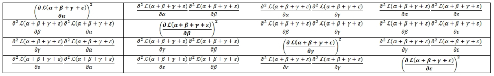
…………Algebraic decomposition of the entries is more common when we’re working with well-defined likelihood formulas, like the one for the normal distribution in Figure 1, which yield the expected Fisher Information through integration. In SQL Server we’re dealing with semi-continuous data, since even our largest data types of course cannot accommodate an infinite number of decimal places; this means we’re essentially limited to the next best thing after integrals, weighed summations over the sample data. This yields the Observed Fisher Information, which is much more tractable. The discrepancy between this and the other idealized version can be leveraged as a sort of goodness-of-fit test, to tell us whether or not our selection of data generating processes was sound.[xxiv] This is in addition to its main use in Design of Experiments (DOE), which I have greatly simplified here. A wide variety of other useful stats with interpretive value can be calculated from the Fisher Information via various matrix operations, many of which are labeled as a type of “optimality” with a letter prefix, such as D-Optimality, E-optimality or T-optimality, which maximize determinants, eigenvalues and traces respectively in order to improve parameter estimates or predictive power.[xxv] A welter of useful alternative interpretations can be attached to Fisher Information, particularly the fact that it represents curvature around the peak of a distribution (and would thus equal zero in the case of perfect certainty).[xxvi] The metric can also be treated as changes in energy or entropy in some cases[xxvii] and the non-diagonals can be viewed as departures from the mean, in proportion to their distance from 0.[xxviii] For data with Gaussian distributions, the MLEs derived from the matrix can be treated as measures of distance much like those covered in the last few articles, since it “is the minimum distance from all potential objects you try to estimate”[xxix]
Beyond Ordinary MLE: Competing Uses and Derivation Methods
The primary use case of estimating the number of records required for an experiment may not be necessary for us, while the discrepancy between the expected and observed versions may not be suited to SQL Server due to the algebraic operations required for the former. I’ve barely scratched the surface of the potential uses here though. Fisher Information is commonly used in physics, but has wide applications in other areas of scientific study. As its Wikipedia entry points out, it is useful in modeling processes in a variety of academic fields, particularly when they exhibit the property of shift invariance (i.e., the results do not change based on the time or order that variables are plugged into the process).[xxx] Fisher Information pops up in unexpected places throughout the data mining literature; for example, while researching my favorite topic, neural nets, I stumbled upon one academic journal article that explains how it converges with Mutual Information (covered in Information Measurement with SQL Server, Part 2.5: Mutual, Lautum and Shared Information) at around 250 neurons.[xxxi] In a previous segment of this series I mentioned how all of the complex interrelationships between the various stochastic information distances can be leveraged to cast a sort of web around the knowledge hidden in our databases, a web which Fisher Information intersects with at key points, thereby strengthening the whole scaffolding of data mining logic. For example, Fisher Information rises and falls in the opposite direction of Shannon’s Entropy and the upper bound of maximum entropy, hence it can be used as a replacement for the latter; this allows researchers to substitute the Principle of Minimum Fisher Information for the Principle of Maximum Entropy when selecting the best models and distributions. This comes in handy because maximum entropy involves exponential calculations, but Fisher Information can be derived from differential equations, which is apparently easier to compute in some circumstances.[xxxii] On the other hand, it has to take into consideration the first derivative, which is not required for Shannon’s Entropy; furthermore, it is “a property that makes it a local quantity (Shannon’s is instead a global one).”[xxxiii]
…………Like most other information measures surveyed in this series, it is intimately related to the topic of Information Measurement with SQL Server, Part 4.1: The Kullback-Leibler Divergence. Basically, it can be interpreted as the curvature of the Kullback-Leibler divergence across families of probability distributions.[xxxiv] For intrepid statistical spelunkers who want to dig deep down to uncharted depth of their data mines, consider that the Fisher Information Metric, an extension of Fisher Information to the cutting-edge field of information geometry, is related to the infinitesimal form of the KL-Divergence across a Riemannian manifold.[xxxv] This enables to us to derive that metric through the alternate means of the second derivative of the Kullback–Leibler.[xxxvi] We can also leverage various interconnections with other topics in this series, such as Shannon’s Entropy, the Jensen-Shannon Divergence and Euclidean Distance, plus others I’m unfamiliar with, like the Wald test[xxxvii], which is apparently used in parameter estimation. The Fisher Information Metric, for example, can be calculated from the Jensen-Shannon merely by dividing its square root by 8.[xxxviii] If we were calculating Fisher Information from data points rather than upon aggregates on our data points, these might represent tempting shortcuts, as was the covariance matrix inversion trick mentioned earlier. Yet if that were the case, we might as well just take the reciprocal of VAR aggregates to determine how much Fisher Information the average row might contain for a particular column.
…………In the long run, we might be able to develop a novel use case for the last scenario that really is adaptable to T-SQL solutions. Fisher Information can be used to derive a complex criterion for judging mining model quality that takes into account goodness-of-fit, dimensionality and geometric complexity simultaneously, under the Minimum Description Length (MDL) principle, which will be the subject of an upcoming installment of this series.[xxxix] Bayesians can also use it to calculate the Jeffreys Prior.[xl] I haven’t been able to experiment with either yet, but it may be possible to simply plug the inverse variances for data points rather than point estimates of aggregates into these formulas. The Matrix also has a handy relationship to itself, in that they can be added together to handle multiple experiments, which “makes it easy to forecast the precision of a joint analysis: just add the Fisher matrices of the experiments, and invert the summed matrix.”[xli] Wittman explains one twist on this, which is to plug Bayesian priors into a covariance matrix and zeros on the diagonals, then invert the result into a Fisher Information Matrix, in the reverse of the normal process; this Matrix can then be added to others for the same set of experiments and the final product can be inverted into a new covariance matrix, to allow us to find the Cramér-Rao Lower Bound for the whole project.[xlii] Bayesian estimation methods (including maximum a posteriori, or MAP) constitute another alternative that I have yet to look into, one that may provide more information, given that MLE amounts to using a “flat prior.”[xliii] One of the challenges with those is the necessity of performing either integration or a weighted sum to derive predictions, whereas in MLE we can simply look at the generated PDF.[xliv] Of course, we can always use the method of moments in place of MLE, if we don’t mind a greater degree of uncertainty. What this boils down to in most cases is falling back on the aggregates derived from our samples, which is a no-brainer. The consensus[xlv] seems to be to use the method of moments instead of MLE when there’s no analytical solution or the computation is otherwise intractable – which is precisely the case if we’re limiting ourselves to coding our point estimates in SQL Server. Upgrading to MLE is no guarantee of success anyways, since it is vulnerable to overfitting,[xlvi] can be confounded when a distribution has multiple modes (i.e. peaks)[xlvii] and is apparently prone to yield wrong answers in challenges like the German Tank Problem.[xlviii] For certain applications, Fisher Information Matrices may also give misleading results in the absence of useful priors.[xlix]
… ………Another twist I looked into in the course of cobbling this article together was simply to populate a table of potential variances, means and counts, then run the likelihood functions in T-SQL on them for demonstration purposes. It’s not terribly difficult to guess the underlying table structure for the code sample below, which I verified against a few dozen rows of MLE practice data I found online for the normal and Bernoulli distributions. At this point, however, it’s quite clear that there’s no practical reason for pursuing it much further. My point that T-SQL can be used quite effectively for various machine learning and data mining uses has been made in past articles, but it doesn’t apply in the case of Fisher Information Matrices, at least if we’re using them for MLE purposes. Fisher Information is a big consideration in the world of information metrics, so I’d be remiss if I left it out of this series entirely – but I’d also be remiss if I didn’t point out that it is a counter-example to my usual refrain about how T-SQL can be quite easily adapted for analytics use cases. Until one of the speculative uses above involving calculations on data points rather than aggregate estimates pans out, we’re better off calculating most or all of our Fisher Information Matrices in other tools, like one of the rapidly proliferating statistical and machine learning libraries available today. That could change quickly if Microsoft adds features or accommodations for matrix math, or new T-SQL routines can be found that overcome the main stumbling block, matrix inversion. If so, it might be possible to put Fisher matrices to use in all kinds of exotic but productive ways, such as detecting data structures and fuzzy sets that might yield the most information, or even setting neural net weights efficiently. Even then we’d still be stuck with some intermediate steps that are unsuitable for SQL Server, like algebraic manipulations, or at least not as efficient, in the case of second partial derivatives. There are many other information measures for us to turn our attention to that really are worth coding in set-based languages like T-SQL.
Figure 3: Simple T-SQL for Practice Point Estimates on Two Distributions
DECLARE @Pi decimal(38,37) = 3.1415926535897932384626433832795028841 — from http://www.eveandersson.com/pi/digits/100
SELECT T2.Mean, T3.Variance,
POWER(2 * @Pi * T3.Variance, –1 * (@Count / CAST(2 as float))) * EXP((-1 / (2 * T3.Variance)) * SUM(POWER(Value1 – T2.Mean, 2))) AS NormalLikelihoodEstimate
FROM Practice.FisherInformationTable AS T1
CROSS JOIN Practice.FisherMLEEstimateTable AS T2
CROSS JOIN Practice.FisherMLEEstimateTable AS T3
WHERE TrialID = @TrialID AND T2.FunctionID =@FunctionID AND T3.FunctionID =@FunctionID
AND Value1 IS NOT NULL
AND T2.Mean IS NOT NULL AND T3.Variance IS NOT NULL
GROUP BY T2.Mean, T3.Variance
ORDER BY NormalLikelihoodEstimate DESC
— the Bernoulli
DECLARE @Count bigint, @SuccessCount bigint
SELECT @Count = COUNT(*)
FROM Practice.FisherInformationTable
WHERE TrialID =3 AND Value1 IS NOT NULL
SELECT @SuccessCount= COUNT(*)
FROM Practice.FisherInformationTable
WHERE TrialID =3 AND Value1 = 1
SELECT T2.ExpectedValue,
Combinatorics.CombinationCountFunction (@Count, @SuccessCount) * POWER(ExpectedValue, @SuccessCount) * POWER(1 – ExpectedValue, @Count – @SuccessCount) AS BernoulliLikelihoodEstimate
FROM Practice.FisherMLEEstimateTable AS T2
WHERE T2.FunctionID =2 AND T2.ExpectedValue IS NOT NULL
GROUP BY T2.ExpectedValue
ORDER BY BernoulliLikelihoodEstimate DESC
See the Wikipedia page “Riemann Sum” at https://en.wikipedia.org/wiki/Riemann_sum
[ii] Shenk, Al, 2008, “Estimating Definite Integrals,” Chapter 6 in E-Calculus, posted March 20, 2008 at the University of California at San Diego web address http://math.ucsd.edu/~ashenk/Section6_6.pdf
[iii] Alvino, Chris, 2017, reply on Mar 14, 2017 to the Quora.com post “Do We Ever Use Maximum Likelihood Estimation?” at https://www.quora.com/Do-we-ever-use-maximum-likelihood-estimation
[iv] On the median as the “maximum likelihood estimator of location” for the Laplacian, see Schoenig, Greg, 2013, reply on July 5, 2013 to the Quora.com thread “How Do You Explain Maximum Likelihood Estimation Intuitively?” at https://www.quora.com/How-do-you-explain-maximum-likelihood-estimation-intuitively
[v] Nejjar, Othman, 2017, reply on Mar 14, 2017 to the Quora.com post “Do We Ever Use Maximum Likelihood Estimation?” at https://www.quora.com/Do-we-ever-use-maximum-likelihood-estimation
[vi] The basic workflow was adapted from Kannu, Balaji Pitchai, 2017, reply on April 7, 2017 to the Quora.com post “How Do You Explain Maximum Likelihood Estimation Intuitively?” at https://www.quora.com/How-do-you-explain-maximum-likelihood-estimation-intuitively
[vii] IBID.
[viii] As always, I use the term loosely to encompass probability mass functions (PMFs) as well, so as not to complicate matters needlessly.
[ix] Chatterjee, Kingshuk, 2017, reply on April 7, 2017 to the Quora.com post “How Do You Explain Maximum Likelihood Estimation Intuitively?” at https://www.quora.com/How-do-you-explain-maximum-likelihood-estimation-intuitively
[x] See the Wikipedia page “Sufficient Statistic” at https://en.wikipedia.org/wiki/Sufficient_statistic Other good sources include the Stat 414/415 course webpages “Lesson 53: Sufficient Statistics” and “Definition of Sufficiency” available the Penn State Eberly College of Science web addresses https://newonlinecourses.science.psu.edu/stat414/node/244/ and https://newonlinecourses.science.psu.edu/stat414/node/282/
[xi] See the Wikipedia page “Fisher Information Metric” at https://en.wikipedia.org/wiki/Fisher_information_metric
[xii] For an introduction, see the Wikipedia page “Bias of an Estimator” at https://en.wikipedia.org/wiki/Bias_of_an_estimator
[xiii] pp. 10-14, Pati contains a good explanation.
[xiv] I usually dislike video tutorials, but I’ve found a couple with powerful illustrations and plain English explanations of the Cramér-Rao Lower Bound and its relationship to likelihood estimates, both by Oxford University tutor Ben Lambert. For example, see Lambert, Ben, 2014, “Maximum Likelihood – Cramer Rao Lower Bound Intuition,” published Feb 20, 2014 at the YouTube web address https://www.youtube.com/watch?v=i0JiSddCXMM and Lambert, Ben, 2013, “The Cramer-Rao Lower Bound: Inference in Maximum Likelihood Estimation,” published Oct 28, 2013 at the YouTube web address https://www.youtube.com/watch?v=igQIsYAlKlY. I have yet to sift through his home page, but it looks like there may be other solid material available there, particularly on likelihood.
[xv] One process for doing so is available on p. 17, Ly, Alexander; Verhagen, Josine; Grasman, Raoul and Wagenmakers, Eric-Jan, 2014, “A Tutorial on Fisher Information,” published September, 2014 at the Alexander-Ly.com web address http://www.alexander-ly.com/wp-content/uploads/2014/09/LyEtAlTutorial.pdf I have not yet had time to evaluate the newer versions now available at the Cornell University arXiv.org web address https://arxiv.org/abs/1705.01064
[xvi] For a succinct example, see the Stat 506 webpage “Lesson 2: Confidence Intervals and Sample Size” at the Penn State Eberly College of Science web address https://newonlinecourses.science.psu.edu/stat506/node/7/
[xvii] For an example, see pp. 7-8,Pati, Debdeep, 2016, “Fisher Information,” published April 6, 2016 at the Florida State University Department of Statistics web address https://ani.stat.fsu.edu/~debdeep/Fisher.pdf
[xviii] Because mathematics and the code that implements it are often that painfully dry as a Saguaro cactus, it is not uncommon for the literature to include brief historical anecdotes on the invention of important concepts, as well as the inventors themselves. I’ve tried to leaven my various amateur mistutorial series with a little of the same, but have been surprised by just how colorful many of the characters have been, if a black heart qualifies as a colorful personality. I have yet to encounter any bizarre anecdotes about Swedish statistician Harald Cramér (1893-1985) and Calyampudi Radhakrishna Rao (1920-present) of Karanataka, India, but then again, they don’t have the same name recognition as R.A. Fisher (1890-1962), the inventor of the Fisher Information Matrix and so many other key statistical innovations like P-Values and analysis of variance (ANOVA). Fisher unfortunately belongs in the same dubious club as René Descartes (1596-1650), who had the charming habit of carrying a mannequin of his dead sister around Europe and talking to it at cafes, or Kurt Gödel (1906-1978), whose fear of poisoning drove him to force his wife to act as his taste-tester (he ended up starving to death when she was hospitalized for other reasons). Like so many of the other “rock star” mathematicians and physicists of old, Fisher was brilliant when he stuck to his own field, but incredibly weak-minded in other ways. For example, “Smoking, he argued, does not cause diseases; it is just that the types of people that smoke also happen to be the types of people that get diseases for other reasons. Maybe these are diseases caused by stress, and stressed people are also more likely to smoke.”[xviii] Like Sir Francis Galton (1822-1911), who I took to task in A Rickety Stairway to SQL Server Data Mining, Algorithm 2: Linear Regression, Fisher was another leading statistician who popularized eugenics among the intelligentsia of Europe, thereby paving the way for the Holocaust. He was not merely a eugenics supporter, but became a Professor of Eugenics at London’s University College in 1933. Even when you factor out its ultimate expression in the Holocaust, it was among the most condescending, arrogant ideas of all time – not only that the government would sterilize etc. the “unfit” but tell people who they could marry and how many children they could breed, so as to produce the most genetically “fit” offspring[xviii]; the irony that Fisher was himself nearly blind and therefore among the “unfit” probably would have been lost on him. By all accounts, Fisher also had a nasty disposition: “He possessed a colossal, overbearing ego, attacking the work of everyone with equal ferocity. He lacked a sense of humor and his colleagues reported that in meetings he would become enraged by some harmless remark that others would merely smile at. Even his disciple Maurice G. Kendall recalled that the character defects Fisher attributed to others were easily discernable in himself. One unnamed colleague stated, “Whenever he paints a portrait, he paints a self portrait.”[xviii] He escalated a dispute with fellow statistical pioneer Karl Pearson into a petty squabble and then a blood feud, which he still prosecuted vindictively 20 years after Pearson was in the ground. Very little of the Information about Fisher is good, but like some of the Nazi scientists brought to America in Operation: Paper Clip, the most constructive thing we can do is salvage something out of the brilliance he demonstrated in his own specialty, by using his tests to reach more accurate conclusions in our DIY data mining experiments. I hate to focus on anyone’s faults, but it should be noted that many of the “rock star” mathematicians and physicists whose names are attached to these inventions were often not just eccentric, but downright frightening.
[xix] Derived from the estimated mean of cells per human body cited in “How Many Cells Are in the Human Body?” at the Wonderopolis web address https://wonderopolis.org/wonder/how-many-cells-are-in-the-human-body
[xx] pp. 6-7, Ly, et al.
[xxi] p. 2, Wittman, David, 2015, “Fisher Matrix for Beginners,” undated monograph published at the University of California UC Davis Department of Physics web address http://www.physics.ucdavis.edu/~dwittman/Fisher-matrix-guide.pdf
[xxii] See the reply on Feb. 22, 2016 by the user named Scortchi to the question “Basic Question on Defining the Dimensions and Entries of the Fisher Information Matrix” at the CrossValidated forum web address http://stats.stackexchange.com/questions/197546/basic-question-on-defining-the-dimensions-and-entries-of-the-fisher-information
[xxiii] See the answer posted Oct. 23, 2013 by the user named prop to the question “What Does the Inverse of Covariance Matrix Say About Data? (Intuitively),” available at CrossValidated forum web address
[xxiv] pp. 8-10, Ly, et al.
[xxv] See the Wikipedia page “Optimal Design” at https://en.wikipedia.org/wiki/Optimal_design “Optimal Design”
[xxvi] See the reply by the user named Neil G to the thread “What Kind of Information is Fisher Information?” on Feb 14, 2016 at the CrossValidated forum web address http://stats.stackexchange.com/questions/196576/what-kind-of-information-is-fisher-information?rq=1. He goes on to say, “If the Fisher information of a parameter is zero, that parameter doesn’t matter. We call ‘information’ because the Fisher information measures how much this parameter tells us about the data.” For an explanation of the curvature, also see the replies to the CrossValidated thread “Intuitive Explanation of a Definition of the Fisher Information” at https://math.stackexchange.com/questions/265917/intuitive-explanation-of-a-definition-of-the-fisher-information
[xxvii] See the Wikipedia entry “Fisher Information Metric” at https://en.wikipedia.org/wiki/Fisher_information_metric
[xxviii] p. 11, Ly, et al.
[xxix] Tung, David, 2015, reply on April 17, 2015 to the Quora.com thread “How Do You Explain Maximum Likelihood Estimation Intuitively?” at https://www.quora.com/How-do-you-explain-maximum-likelihood-estimation-intuitively
[xxx] See the Wikipedia pages “Fisher Information” at http://en.wikipedia.org/wiki/Fisher_information, “Shift-Invariant System” at https://en.wikipedia.org/wiki/Shift-invariant_system and “Time-Invariant System” at https://en.wikipedia.org/wiki/Time-invariant_system
[xxxi] Yarrow, Stuart and Challis, Edward, 2012, “Fisher and Shannon Information in Finite Neural Populations,” pp. 1740-1780 in Neural Computation, July 2012. Vol. 24, No. 7. Available online at The University of Edinburgh School of Informatics web address
http://homepages.inf.ed.ac.uk/pseries/pdfs/YarrowChallisSeries_NC.pdf
[xxxii] See the Wikipedia page “Minimum Fisher Information” a http://en.wikipedia.org/wiki/Minimum_Fisher_information
[xxxiii] IBID.
[xxxiv] See the Wikipedia pages “Fisher Information” at http://en.wikipedia.org/wiki/Fisher_information and “Kullback Leibler Divergence” at http://en.wikipedia.org/wiki/Kullback%E2%80%93Leibler_divergence
[xxxv] See the Wikipedia page “Fisher Information Metric” at https://en.wikipedia.org/wiki/Fisher_information_metric
[xxxvi] IBID.
[xxxvii] See the Wikipedia page “Fisher Information” at http://en.wikipedia.org/wiki/Fisher_information
[xxxviii] See the Wikipedia page “Fisher Information Metric” at https://en.wikipedia.org/wiki/Fisher_information_metric
[xxxix] p. 29, Ly, Alexander; Verhagen, Josine; Grasman, Raoul and Wagenmakers, Eric-Jan, 2014, “A Tutorial on Fisher Information,” published on the personal webpage of Eric-Jan Wagenmakers at http://www.ejwagenmakers.com/submitted/LyEtAlTutorial.pdf
[xl] IBID, pp. 22-26.
[xli] p. 8, Wittman.
[xlii] IBID., p. 7.
[xliii] See the replies by Michael Hochster on Dec 11, 2013 and Zare, Hadi on Oct. 22, 2015 to the Quora.com thread “What is the Difference Between Bayesian Estimation and Maximum Likelihood Estimation” at https://www.quora.com/Intuitively-speaking-What-is-the-difference-between-Bayesian-Estimation-and-Maximum-Likelihood-Estimation
[xliv] See the replies by Albert Wu on Oct. 27, 2015 and Fayi Femi-Balogun, May 24, 2015 to the Quora.com thread “What is the Difference Between Bayesian Estimation and Maximum Likelihood Estimation” at https://www.quora.com/Intuitively-speaking-What-is-the-difference-between-Bayesian-Estimation-and-Maximum-Likelihood-Estimation
[xlv] See the Quora.com thread “When Should Method of Moments Be Used Instead of Maximum Likelihood Estimation for Point Estimates?” at https://www.quora.com/When-should-method-of-moments-be-used-instead-of-maximum-likelihood-estimation-for-point-estimates
[xlvi] Baisero, Andrea, 2013, reply on Dec. 22, 2013 to the Quora.com thread “How Do You Explain Maximum Likelihood Estimation Intuitively?” at https://www.quora.com/How-do-you-explain-maximum-likelihood-estimation-intuitively
[xlvii] See the reply by J.Q. Veenstra on Nov. 5, 2015 to the Quora.com thread “What is the Difference Between Bayesian Estimation and Maximum Likelihood Estimation” at https://www.quora.com/Intuitively-speaking-What-is-the-difference-between-Bayesian-Estimation-and-Maximum-Likelihood-Estimation
[xlviii] See the reply by Bill Bell on March 15, 2015 to the Quora.com thread “When Might Maximal Likelihood Estimation Fail?” at https://www.quora.com/When-might-maximal-likelihood-estimation-fail Also see Smith, David, 2010, “German Tanks, Statistical Intelligence,” posted May 25, 2010 at the Revolution Analytics blog address https://blog.revolutionanalytics.com/2010/05/german-tanks-statistical-intelligence.html
[xlix] Vallisneri, Michele, 2008, “Use and Abuse of the Fisher Information Matrix in the Assessment of Gravitational-wave Parameter-estimation Prospects,” pp. 042001:1-20 in Physical Review, Feb. 4, 2008. Vol. 77, No. 4. Available online at the NASA Jet Propulsion Laboratory web address http://authors.library.caltech.edu/9589/1/VALprd08.pdf Also see Vallisneri, Michele, 2007, “A User Manual for the Fisher Information Matrix,” monograph published Feb. 9, 2007 at the LIGO Scientific Collaboration web address http://www.ligo.org/pdf_public/P070009-00.pdf
