By Steve Bolton

…………“The shortest distance between two points is a straight line.”
…………In this famous remark, Archimedes[1] (287-212 B.C.) managed to sum up all of the uses for Euclidean Distance, i.e. the way that laymen and data scientists ordinarily use to measure ranges of space on a daily basis. Beatnik poet Charles Bukowski may have unwittingly summed up all of the reasons for alternate spatial measures in his much more entertaining quote, “The shortest distance between two points is often unbearable.”[2] For example, the notion of curved space has percolated down somewhat from astrophysics and quantum theory down to the public, through the aid of science media like the Discovery Channel and PBS’ Nova program. Data science and information theory likewise require specialized measures of distance, which can be used to gauge the similarity or dissimilarity of data points, or applied to their probabilities, entropies, predicted values, Z-Scores and other such information that can be attached to them. The reason why is best encapsulated by the single example of Manhattan Distance, which was developed to answer a very practical question that we all might encounter: how do we gauge the distance we must travel if we’re limited to following a grid pattern, instead of taking straight lines to our destinations? Analysts often encounter more complicated use cases where more sophisticated measures are called for, such as measuring the distance between probability distributions using the means outlined in the last two articles. I also introduced Shared Information Distance earlier in this series of mistutorials (which I am entirely unqualified to write) and already tackled Cook’s Distance and Mahalanobis Distance in a previous series, Outlier Detection with SQL Server. In the next six articles in this segment of the Information Measurement series I’ll be covering several families of alternative measures commonly used in information theory and data science (particularly in clustering algorithms), but they ought to be a breeze, given that we’ve already gotten the most difficult measures out of the way. The good news is that it’s not particularly difficult to calculate any of the measures I’ll introduce in this segment, many of which can implemented in T-SQL code that run on multi-million-row datasets in milliseconds.
…………To grasp the need for applying different distance measures to DIY data mining scenarios, think of the vision tests given by optometrists. As they flip through various choices of lenses using phoropters, each distorts our view of the eye charts in distinctive ways; only one choice of lens will lead to maximum clarity of vision. Likewise, when judging things like the distance between data points or probability distributions, we often need to carefully select a metric that will properly bring the underlying information into focus, for the same reason that hawks need sharp vision to locate prey, whereas rabbits need stereoscopic vision to escape them. I’m using the term “metric” loosely here; as I pointed out in the first articles of this segment, on the Kullback-Leibler and Jensen-Shannon Divergences, it technically means a measure that possesses four mathematical properties, including subadditivity, symmetry, positivity and positive definiteness. A true “distance” in the professional sense doesn’t possess subadditivity, while a divergence is also missing symmetry. The usefulness of particular metrics, distances and divergences in dictated largely by these and other properties, some of which can be deleterious; for example, as we saw two articles ago, the property of absolute continuity disqualifies the use of the Kullback-Leibler Divergence in comparing many sets of probability distributions. The properties exhibited by these measures in turn flow from the underlying math formulas. There are literally hundreds of available distance measures, so I can’t possibly tackle all of them, or even explain all of the ways of organizing them into different taxonomies. Instead, I’ll stick with the methodology used by Cha Sung-Hyuk, who grouped probabilistic distances into eight families in an excellent article for the International Journal of Mathematical Models and Methods in Applied Sciences in 2007.[3]  I highly recommend this well-written source for the underlying equations, as well as Deza’s Dictionary of Distances, which was also of immense help in writing this segment of the series.[4]
…………I usually leave the underlying equations out of these discussions on the grounds that they are incredibly useful for helping theoreticians communicate within one another, but a real hindrance to end users of data mining software; just as a biker shouldn’t have to give a dissertation on motorcycle engineering to attend the Sturgis rally, so too should data miners be freed from the implementation details of mining software as much as possible. Nevertheless, it is immediately obvious (even to someone with rusty math skills like me) why the equations for the Minkowski Family of distance are so similar. At the heart of all four is a simple subtraction of one data point or probability from another, with a few simple tweaks; SQL Server users may find it easier to grasp this from the sample T-SQL in Figure 1, which begins with three common table expressions (CTEs) that are all ultimately boil down to the DifferenceAmount bubbled up from the CrossProductCTE. The DifferenceAmount is calculated from a simple comparison of the raw values of the first and second float columns[5] in the 11-million-row Higgs Boson dataset[6], which I’ve found handy for stress-testing my T-SQL data mining samples in this series and others prior to it. The SELECT that follows the three CTEs merely performs simple aggregates like SUMs or MAXs on the various differences that emerge from them. In the next SELECT, I calculate the Euclidean Distance by taking the root of the Squared Euclidean Distance, which is then used to derive a handy EuclideanRatio in the last. Euclidean Distance is a good first choice when matching metrics to particular use cases, thanks to its simplicity, but as I mentioned above, some scenarios may call for nuanced measures like Manhattan Distance. Squared Euclidean Distance can be used “to place progressively greater weight on objects that are farther apart,”[7] but it comes at the cost of the desirable property of subadditivity[8], as well as extra computational overhead[9]. It is easy to see how the two Euclidean types are related, but the linkages between the Euclidean, Manhattan (a.k.a. the “City Block” or “Taxicab” distance) and Chebyshev distances are only fully apparent when we factor in the Minkowski Distance, which subsumes them all. Grouping them together is justified not just by the similarities in the underlying mechanics, but by the fact that we can derive the Manhattan Distance by plugging a value of 1 into the Minkowski Distance parameter, or the Euclidean Distance using a value of 2. As the values of the parameter increase, they approach the ultimate limit represented by the Chebyshev Distance, which measures the greatest possible distance along any axis. Plugging in a value of 0 will naturally produce a divide-by-zero error, since SQL Server – like almost all modern software – still can’t represent infinity, which is the true result of such operations. It is all quite similar to the way in which the Rényi and Gibbs Entropies return various other common entropies, as explained in Information Measurement with SQL Server, Part 2.2: The Rényi Entropy and Its Kin and Information Measurement with SQL Server, Part 2.3: Thermodynamic and Quantum Entropies. Formulas are also available to generalize the Minkowski Family to mathematical structures known as L_k-norms, but I won’t complicate things needlessly by explaining how its K parameter returns the corresponding Euclidean or Manhattan norms.[10] My main goal in this segment is to demonstrate how easy it is to implement your own distance measures in SQL Server for DIY data mining purposes, not delve into higher-level math structures. With some sprucing up, code like this could be used to derive your own DIY clustering algorithms that can be displayed in Reporting Services, among other uses.

Figure 1: Sample T-SQL for Calculating the Minkowski Family of Distances
DECLARE @EuclideanDistance float,
@SquaredEuclideanDistance float,
@ManhattanDistance float,
@MinkowskiDistance float,
@ChebyshevDistance float,
@ChiSquaredDistance float,
@AverageOfCityBlockAndChebyshevDistances float

DECLARE @Count bigint, @MinkowskiDistanceParameterfloat  = 1

SELECT @Count=Count(*)
FROM Physics.HiggsBosonTable
WHERE Column1 IS NOT NULL

; WITH TempCTE
(PK, Value1, Value2)
AS
(SELECT TOP 999999999999999 ID, CAST(Column1 AS float) AS Value1, CAST(Column2 AS float) AS Value2
FROM Physics.HiggsBosonTable
WHERE Column1 IS NOT NULL AND Column2 IS NOT NULL
ORDER BY ID
),
CrossProductCTE
(PK, Value1, Value2, SquaredDifference, AbsoluteDifference, MinkwoskiDifference, ChiSquareDifference)
AS
(SELECT PK,  Value1, Value2,
Power(DifferenceAmount, 2) AS SquaredDifference,
Abs(DifferenceAmount) AS AbsoluteDifference,
Power(Abs(DifferenceAmount), @MinkowskiDistanceParameter) AS MinkwoskiDifference,
CASE WHEN Value1 + Value2 = 0 THEN 0 ELSE Power(DifferenceAmount, 2) / Power(Value1 + Value2, 2) END AS ChiSquareDifference
FROM
(SELECT PK, Value1, Value2, Value1 – Value2 AS DifferenceAmount
       FROM TempCTE) AS T1
),
MaxAbsouteDifferenceCTE
(MaxAbsoluteDifference)
AS
(
SELECT Max(AbsoluteDifference) AS MaxAbsoluteDifference
       FROM CrossProductCTE
)

SELECT @SquaredEuclideanDistance = Sum(SquaredDifference),
@ManhattanDistance = SUM(AbsoluteDifference),
@MinkowskiDistance = Power(SUM(MinkwoskiDifference), (1 / @MinkowskiDistanceParameter)),
@ChebyshevDistance = MaxAbsoluteDifference ,
@ChiSquaredDistance= SUM(ChiSquareDifference),
@AverageOfCityBlockAndChebyshevDistances = SUM(AbsoluteDifference + MaxAbsoluteDifference) / 2
FROM CrossProductCTE AS T1
      INNER JOIN (SELECT MaxAbsoluteDifference FROM MaxAbsouteDifferenceCTE) AS T2
       ON 1 = 1
GROUP BY MaxAbsoluteDifference

SELECT @EuclideanDistance = Power(@SquaredEuclideanDistance, 0.5)

SELECT @EuclideanDistance AS EuclideanDistance, @EuclideanDistance / CAST(@Count as float) as EuclideanRatio,
@SquaredEuclideanDistance AS SquaredEuclideanDistance,
@SquaredEuclideanDistance  / CAST(@Count as float) as SquaredEuclideanRatio,
@ManhattanDistance AS ManhattanDistance,
@ManhattanDistance / CAST(@Count as float) as SquaredManhattanRatio,
@MinkowskiDistance AS MinkowskiDistance,
@ChebyshevDistance AS ChebyshevDistance,
@ChiSquaredDistance AS ChiSquaredDistance,
@AverageOfCityBlockAndChebyshevDistances AS AverageOfCityBlockAndChebyshevDistances

 Figure 2: Calculating a Range of Values for the Minkowski Parameter
— A WHOLE RANGE OF MINKOWKSI DISTANCES
SELECT MinkowskiDistanceParameter, Power(SUM(Power(CAST(Abs(Column1 – Column2) as float), MinkowskiDistanceParameter)), 1 / CAST(MinkowskiDistanceParameter as float)) AS MinkowskiDistance
FROM (VALUES (0.5), (1),(2), (3), (4),(5), (10), (50)) AS T1(MinkowskiDistanceParameter)
LEFT JOIN  Physics.HiggsBosonTable AS T2
       ON 1 = 1
WHERE Column1 IS NOT NULL AND Column2 IS NOT NULL
GROUP BY MinkowskiDistanceParameter
ORDER BY MinkowskiDistanceParameter

 Figure 3: Results from the Higgs Boson Dataset (click to enlarge)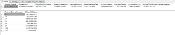

…………As expected, the Euclidean and Manhattan Distances pop out of the Minkowski formula in Figure 2 when the right parameters are plugged in. As the parameter values rise from 0.5 to 1 through 5, then 10, then 50, the results approach the Chebyshev Distance but never quite reach it. Without this additional code, the query runs in 23 seconds on my wheezing desktop development machine; in next month’s article (a timetable that assumes I won’t break my hand again like I did this summer, the culprit behing the long hiatus in this blog series), I’ll demonstrate how to reduce this to a matter of milliseconds by precalculating standardized values. The execution plans were nice and boring, just like we like ‘em: there were only two queries, the second of which accounted for 97 percent of the batch costs, and within that there were only 16 operators, grouped into two chains brought together in a Nested Loop. Each chain began with two Index Seeks and the Sort operators within those chains accounted for 69 percent of the query costs, so there apparently isn’t much room for optimization – unless we do precalculated standardization, which can be done on the same tables in just 3 seconds and used to derive even more sophisticated distances in milliseconds, as I discovered to my surprise when writing the rest of the articles in this segment. In fact, my omission of scaling would render the comparisons of these particular Higgs Boson columns nonsensical. Because the first ranges from -0.9999616742134094238 to 12.09891414642333984 and the second from -2.434976100921630859 to 2.43486785888671875, it is likely that we’re making apples-and-oranges comparisons between objects on different scales, which will distort – but not entirely invalidate – the resulting distances. It would be much easier to interpret these distance values if the underlying data points were on the same scale, as they are when we compare probabilities, which are always on a scale of 0 to 1. One of the most popular ways of scaling is to subtract each value from the column’s mean and then divide by the standard deviation[11], but I have had better luck with the methods I introduced in the previous tutorial series, Implementing Fuzzy Sets in SQL Server.
…………Since I’m an amateur who writes these tutorials merely to grasp the material faster, I like to lace my articles with more disclaimers than a pharmaceutical commercial. I was able to validate some of these common measures through such means as comparing them to the Minkowski Distance at various parameter values, but some of the more advanced distances I’ll cover in the next five articles are more difficult to check for accuracy. This includes the Chi-Squared Distance included in the sample code above. It is something of an oddball metric, for which the documentation is comparatively thin (although I have seen it mentioned several times in texts on information theory, particularly in reference to quantum information). It is also used for “used in correspondence analysis and related ordination techniques” but has its detractors when used as a tool in ecology.[12] The formula involves dividing the squared difference by the squared sum of values[13], which resembles the inner workings of the some of the other metrics I’ll delve into in the next few articles. I won’t be covering the Pearson Correlation Coefficient, which has a similar formula but is more often performed on Z-Scores and has the count as the divisor.[14] It is not included in Sung-Hyuk’s really useful taxonomy, but it equal to half of the value of one measure in the L2 family, most of which involve division operations with differences and sums in the divisors. Most of the measures in that family have Chi-Squared (i.e. ?²) in their names. I included it within the Minkowski Family because of its dependence on the difference operation, but it seems to straddle the line between the Minkowski and L₂ families, as well as next week’s topic, the L₁ group. Some of its most commonly used members include the Sørensen and Canberra metrics, which also resemble the Chi-Squared Distance, except that the dividend and divisor are squared. Both the L₁ and L₂ build upon Euclidean Distance and its relatives by incorporating either the Euclidean or Squared Euclidean Distance in their definitions, thereby allowing us to derive alternative mathematical properties that can be leveraged to meet more sophisticated use cases than merely measuring a straight line between two points, or along right angles as the Manhattan Distance does. This time around I left out scaling[15] in order to keep things light and simple, but in the next installment we’ll see how we can improve both the performance and interpretability of these distance metrics through proper scaling, which is a win-win bargain.

1 Its origins are widely attributed to Archimedes, including at webpages like Lombaro, Crystal R., 2014, “21 Famous Archimedes Quotes,” published Dec 12, 2014 at the NLCATP.org web address http://nlcatp.org/21-famous-archimedes-quotes/

2 See the undated Goodreads.com webpage “Charles Bukowski” at http://www.goodreads.com/quotes/27469-the-shortest-distance-between-two-points-is-often-unbearable

3 Sung-Hyuk, Cha, 2007, “Comprehensive Survey on Distance/Similarity Measures between Probability Density Functions,” pp. 300-307 in International Journal of Mathematical Models and Methods in Applied Sciences, Vol. 1, No. 4.

4 Deza, Elena and Deza, Michel Marie, 2006, Dictionary of Distances. Elsevier: Amsterdam.

5 These were floats in the original dataset, but I was able to cut them down to decimal(33,29) without losing any precision.

6 I downloaded this in 2014 from the University of California at Irvine’s Machine Learning Repository and converted it into a SQL Server table, which occupies about 6 gigs of space in a DataMiningProjects database.

7 See the Wikipedia webpage “Euclidean Distance” at http://en.wikipedia.org/wiki/Euclidean_distance#Squared_Euclidean_distance

8 See the reply by Cook, Bill to the StackExchange Mathematics thread “Euclidean Distance Proof” posted at http://math.stackexchange.com/questions/75207/euclidean-distance-proof on Oct. 23, 2011.

9 In some clustering applications, it may cost more to derive the Euclidean from the root of the Squared Euclidean Distance; I seem to do the same in my T-SQL sample, but if you look carefully, my Squared Euclidean is ultimately derived from a POWER operation which can be omitted if all we need is the Euclidean. See the undated webpage “Overview: Euclidean Distance Metric” at the Improved Outcomes Software address http://www.improvedoutcomes.com/docs/WebSiteDocs/Clustering/Clustering_Parameters/Euclidean_and_Euclidean_Squared_Distance_Metrics.htm

10 For an introduction to the concept of norms, see Scarfboy, 2014, “Similarity or Distance Measures,” published March 5, 2014, at the Knobs-Dials.com web address  http://helpful.knobs-dials.com/index.php/Similarity_or_distance_measures and the Wikipedia page “Norm (Mathematics)” http://en.wikipedia.org/wiki/Norm_%28mathematics%29#Euclidean_norm

11 Palmer, Mike, 2015, “Statistics,” undated webpage published at the Ordination Methods for Ecologists web address http://ordination.okstate.edu/STATS.htm

12 pp. 9-50, McCune, Bruce; Grace, James B. and Urban, Dean L., 2002, Analysis of Ecological Communities. MjM Software Design: Gleneden Beach, Oregon.

13 “As d(x,y) = sum( (xi-yi)^2 / (xi+yi) ) / 2, where x and y are your histograms, and i is the bin index of the histogram.” See the reply by Singh, Bharat to the StackOverflow thread “Calculate Chi-squared Distance Between Two Image Histograms in Java,” published July 30, 2014  at http://stackoverflow.com/questions/25011894/calculate-chi-squared-distance-between-two-image-histograms-in-java. Also see the reply by Kemmler, Michael to the ResearchGate thread “What is Chi-squared Distance? I Need Help With the Source Code,” published Jan 7, 2013 at http://www.researchgate.net/post/What_is_chi-squared_distance_I_need_help_with_the_source_code

14 See the  undated webpage “Pearson Correlation and Pearson Squared” at the Improved Outcomes Software address http://www.improvedoutcomes.com/docs/WebSiteDocs/Clustering/Clustering_Parameters/Pearson_Correlation_and_Pearson_Squared_Distance_Metric.htm

15 Singh and Kemmler both mention that the Chi-Squared Distance really ought to be binned, which I have not done here but will in the articles that follow.