

By Steve Bolton
…………In the first installment of this wide-ranging series of amateur tutorials, I noted that the Hartley function indeed returns “information,” but of a specific kind that could be described as “newsworthiness.” This week’s measure also quantifies how much we add to our existing knowledge from each new fact, but through explicitly stochastic methods, whereas the Hartley function is more closely related to counts of state descriptions than probabilities.[1] Shannon’s Entropy is of greater renown than its predecessor, but isn’t much more difficult to code in T-SQL. In fact, it should be a breeze given that I already posted a more advanced version of it tailor-made for Implementing Fuzzy Sets in SQL Server, Part 10.2: Measuring Uncertainty in Evidence Theory, just as I had already coded a modified version of Hartley’s measure for Implementing Fuzzy Sets in SQL Server, Part 9: Measuring Nonspecificity with the Hartley Function.
…………Historically, the real difficulty with the metrics of information theory is with their interpretation, largely due to the broad and fuzzy meaning of the imprecise term, “information.” As we shall see, many brilliant theorists far smarter than we have made the mistake of overextending it beyond its original domain, just as some thinkers have gotten carried with the hype surrounding fuzzy sets and chaos theory. Like those cutting-edge topics, Shannon’s Entropy and its relatives within information theory are indeed powerful, but can go badly wrong when misapplied outside its specific use cases. It has really subtle yet mind-blowing implications for all of the different classes of information measurement I hope to cover in this wide-ranging and open-ended series, not all of which are fully understood. My purposes in this series is to illuminate datasets from every possible direction, using a whole smorgasbord of measures of meaning (semantic information), randomness, complexity, order, redundancy and sensitivity to initial conditions, among others; since many of these metrics serve as the foundation of many mining algorithms, we can use them in a SQL Server environment to devise DIY data mining algorithms. Shannon’s Entropy intersects many of these disparate class of information in multifarious ways, such as the fact that it is equal to the Hartley measure in the case of uniform distributions (i.e. when all values are equally likely). It is not a measure of what is known, but of how much can be learned by adding to it; entropy measures rise in tandem with uncertainty precisely we because we can learn more from new facts when we don’t already know everything. It can thus be considered complementary to measures of existing knowledge, such as Bayes Factors. I’ve read more on information theory than many other fields I’ve commented on over the past couple of years, when I started writing self-tutorials on data mining, but that doesn’t mean I understand all of these complex interrelationships well. In fact, I’m writing this series in part because it helps me absorb the material a lot faster, and posting it publicly in the hopes that it can at least help readers avoid my inevitable mistakes. I lamented often in A Rickety Stairway to SQL Server Data Mining that SSDM was woefully under-utilized in comparison to its potential benefits, but the same can also be said of the algorithms that underpin it.
Channel Capacity as a Godsend
Few of these information metrics are as well-known as the measure that Claude E. Shannon (1916-2001), a key American cryptographic specialist during the Second World War, introduced in 1948 in a two-part journal article titled “A Mathematical Theory of Communication.”[2] Most of it consists of math theorems and formulas that only got thicker as researchers built on his theory over the years, but it is noteworthy to mention that he credits earlier work by electrical engineers Ralph Hartley[3] (1888-1970) and Harry Nyquist (1889-1976) in the opening paragraphs.[4] I’ll skip over most of the proofs and equations involved – even the ones I understand – for the usual reasons: as I’ve pointed out in past articles, users of mining tools shouldn’t be burdened with these details, for the same reason that commuters don’t need a degree in automotive engineering in order to drive their cars. Suffice it to say that the original purpose was to determine the shortest possible codes in the case of noisy transmission lines. In this effort to extend coding theory, Shannon gave birth to the whole wider field of information theory. Masud Mansuripur, the chair of the Optical Data Storage Department at the University of Arizona, sums up Shannon’s surprising mathematical discovery best: “In the past, communications engineers believed that the rate of information transmission over a noisy channel had to decline to zero, if we require the error probability to approach zero. Shannon was the first to show that the information-transmission rate can be kept constant for an arbitrarily small probability of error.”[5] It is also possible to determine the information-carrying capacity of the channel at the same time.[6]
…………The idea is still somewhat startling to this day, as many writers in the field of information theory have pointed out ever since; it almost seems too good to be true. Basically, the idea is to engineer a “decrease of uncertainty as to what message might have been enciphered,” [7] in part by leveraging combinatorics to derive probabilities. For example, the Law of Large Numbers states that rolling a pair of dice is far more likely to result in a number like eight, since there are multiple ways of adding up both dice to get that result, whereas there’s only one combination apiece for snake eyes or boxcars. The edges of the resulting dataset are thus far less likely than the values in the middle, just as we’d find in a Gaussian or “normal” distribution, i.e. the ubiquitous bell curve. This gives rise to a dizzying array of axioms and lemmas and a whole set of procedures for determining codes, all of which I’ll skip over. For perhaps the first time in the history of this blog, however, I have a sound reason for posting the underlying equation: H = -S pi logb pi. It’s not a household name like E = mc2 or 2 + 2 = 4, but it’s still one of the most famous formulas of all-time. It relatives can be spotted in the literature by the telltale combination of a negative summation operator with a logarithm operation. Aside from the fact that it possesses many ideal mathematical properties[8], “it was proven in numerous ways, from several well-justified axiomatic characterizations, that this function is the only sensible measure of uncertainty in probability theory.”[9]
Translating H into Code
As with Hartley’s measure, a base 10 logarithm results in units known as hartleys or bans (as famed cryptographer Alan Turing called them). With Euler’s Number (as in the natural logarithm) the units are known as nats and with base 2, they’re referred to as shannons or more commonly, bits. The code in Figure 1 uses bits, but users can uncomment the numbers that follow to use one of the other units. It is also worth noting that physicist Léon Brillouin used a “negentropy” measure that is basically the inverse of H, to compensate for the fact that Shannon’s Entropy measures information in terms of uncertainty, which is a bit counter-intuitive; it never really caught on though.[10]
…………My sample code derives some fake probabilities by taking the known proportions of values for a column in the same Higgs Boson dataset[11] I’ve been using for practice purposes for several tutorial series. The probabilities are then multiplied by the logs for those probabilities, then summed across the dataset and multiplied by -1. It’s actually quite simpler than it looks; the table variable and INSERT statement could be done away with altogether if we already had probability figures calculated through some other means, such as some sort of statistical sampling method or even reasoning out the probabilities from the underlying process, as writers on information theory often do with dice and cards to illustrate the concepts. In fact, if we know the underlying probability distribution in advance, we can sometimes calculate the entropy in reverse by using special formulas specific to certain distributions, such as the normal. Moreover, all of the code pertaining the @UniformProportion is included solely for the purpose of validating the results, which equal the results we received in the last article for the DISTINCT version of the Hartley function, as expected. If need be, users can also validate their results using Lukasz Kozlowski’s Shannon Entropy Calculator. All of that can code can also be removed at will. Despite all of this extraneous baggage, the code ran in just 1.9 seconds according to the Client Statistics, on 11 million rows of float values on my beat-up, wheezing semblance of a development machine. The execution plan was uneventful and consisted mainly of seeks on the nonclustered index I put on the column a couple of tutorial series ago.
Figure 1: Shannon’s Entropy in T-SQL
DECLARE @LogarithmBase decimal(38,36) = 2 –2.7182818284590452353602874713526624977 — 10
DECLARE @Count bigint, @DistinctValueCount bigint, @ShannonsEntropy float, @EntropyForUniformDistribution float,
@MaxProbability float, @ChebyshevEntropy float, @MetricEntropy float, @UniformProportion float
SELECT @Count = Count(*), @DistinctValueCount = Count(DISTINCT Column1)
FROM Physics.HiggsBosonTable
WHERE Column1 IS NOT NULL
SELECT @UniformProportion = 1 / CAST(@DistinctValueCount as float)
FROM Physics.HiggsBosonTable
WHERE Column1 IS NOT NULL
DECLARE @EntropyTable table
(Value decimal(33,29),
ValueCount bigint,
Proportion float,
SelfInformation float
)
INSERT INTO @EntropyTable
(Value, ValueCount, Proportion, SelfInformation)
SELECT Value, ValueCount, Proportion, –1 * Proportion * Log(Proportion, @LogarithmBase) AS SelfInformation
FROM (SELECT Value, ValueCount, ValueCount / CAST(@Count AS float) AS Proportion
FROM (SELECT Column1 AS Value, Count(*) AS ValueCount
FROM Physics.HiggsBosonTable
WHERE Column1 IS NOT NULL
GROUP BY Column1) AS T1) AS T2
SELECT * FROM @EntropyTable
SELECT @ShannonsEntropy = SUM(SelfInformation), @EntropyForUniformDistribution= SUM (@UniformProportion * Log(@UniformProportion, @LogarithmBase)) * –1, @MaxProbability = Max(Proportion)
FROM @EntropyTable
— ====================================
— SOME RELATED ENTROPIES
— ====================================
SELECT @ChebyshevEntropy = –1 * Log(@MaxProbability, @LogarithmBase)
SELECT @MetricEntropy = @ShannonsEntropy / CAST(@Count as float)
SELECT @ShannonsEntropy AS ShannonsEntropy, @MetricEntropy AS MetricEntropy, @ChebyshevEntropy AS ChebyshevEntropy, @EntropyForUniformDistribution as EntropyForUniformDistribution
Figure 2: Calculating Shannon’s Entropy on the Higgs Boson Dataset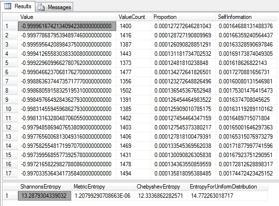
…………Note that in the last section of the code, I tacked on the Metric and Chebyshev Entropies, which are trivial to calculate once we have building blocks like Shannon’s Entropy. References to the Chebyshev Entropy[12], a.k.a the Min Entropy because it represents the minimum amount a variable can exhibit, seem to be few and far between outside the realm of quantum physics. Metric Entropy, on the other hand, can serve as a simple measure of randomness[13], which is more likely to be useful to SQL Server users. These are among a couple dozen extensions and relatives of Shannon’s Entropy, a few of which I’ve already dealt with, like the Hartley Entropy (i.e. the Max Entropy). I won’t discuss Differential Entropy, the extensions to continuous variables using various methods of calculus, because SQL Server data types like float, decimal and numeric are actually discrete in the strict sense; they can’t actually represent infinitesimal grades in between values, any more than the data types of any other software can on finite computers. Nor will I delve into the myriad applications that have been developed from Shannon’s Entropy for signal transmission and coding theory, since these are off-topic.
Detection of “Randomness” and Other Uses
Its relationship to cryptography might be a more appropriate subject, but for the sake of brevity I’ll limit my discussion to pointing out how it sheds light on the nature of “randomness.” Like “information,” it’s a broad term that raises the danger of “definition drift,” even within one’s own mind; I’ve seen big names in certain scientific fields unconsciously shift their usage of the term from “unintentioned” to “uncaused” to “indeterminate” and back again, without discerning the subtle differences between them all. In data mining, we’re basically trying to uncover information that is badly concealed, whereas in cryptography it’s deliberately concealed by mixing it in with apparently random information; the patterns generated by cryptographers are the opposite of random in one specific sense, that it takes great intelligence and hard work to deliberately create these false patterns. Cryptanalysis involves detecting these deliberate patterns, in order to remove the noise obscuring the original message. Of course, “noise” is a subjective matter determined entirely by the questions we choose to ask of the data (although the answers to those questions are entirely objective). Randomness can thus be viewed as excess information of the wrong kind, not an absence of pattern or lack of causation. For example, if we’re looking for evidence of solar flares, then the static on shortwave radios might tell us a lot, but if we’re trying to listen to a broadcast from some foreign land (like the mysterious “numbers stations,” which I picked up when I was younger) then it degrades our information. Consider the case of paleontologists trying to follow dinosaur tracks: each rain drop that has fallen upon them over the eons has interfered with that pattern, but the rain itself follows a pattern, albeit the wrong kind. It is only random for our chosen purposes and pattern recognition goals, but perhaps not to some prehistoric weathermen to whom the pattern of rain might’ve been of keen interest. The relationship between randomness and information is thus quite deep; this brief introduction is merely a wade into the kiddie pool. Later on in this series we may have to dive in, if the measures of randomness I hope to discuss call for it.
…………Shannon’s Entropy and related concepts from information theory have all sorts of far-flung implications, some of which are understood in great detail (particularly when they relate directly to designing codes with minimum information loss) and others which are really intellectually challenging. One of the simplest yet trickiest rules is that the greater the uncertainty, the greater the amount of probabilistic information that can be conveyed with each new record. [14] Some of the corollaries of information theory can be put to good use in reasoning from the data we’ve mined, which is after all, its raison d’etre. The principle of maximum entropy, for example, states that the ideal probability density functions (PDFs) maximize Shannon’s Entropy when producing the expected values.[15] I’d imagine that this could be leveraged for such good purposes as mining model selection. There are all kinds of hidden relationships to other forms of information I hope to cover eventually, such as redundancy, which is a big topic within coding theory. Someday I hope to tackle measures of semantic information, which can be extremely difficult to grasp because they quantify the actual meaning of data, which can be quite slippery. Sometimes the absence of any data at all can tell us everything we need to know, which many mystery writers and crime scene investigation shows have put to good use. More often, people often differ not only between but within themselves as the meaning they choose to assign to terms and numbers, without thinking it through clearly. Perhaps this would make it an ideal field to apply fuzzy sets to, since their chief use cases include modeling imprecision in natural language, as I discussed ad nauseum in the last tutorial series.
Semantic Misinterpretation, Cybernetics, “Disorder” and Other Subtle Stumbling Blocks
Shannon’s Entropy is probably further away from semantic information than fuzzy sets, but that hasn’t stopped many theorists from mistakenly conflating stochastic information with meaning. Shannon himself warned against this kind of bandwagon-jumping.[16] In fact, that’s probably the most common stumbling block of all. Perhaps the clearest cautionary tale is the whole philosophy developed out of information theory by bombastic mathematician Norbert Wiener (1894-1964), who asserted explicitly and deliberately” the very same connection to semantic meaning that Shannon and others cautioned against.[17] Another great mathematician who took Shannon’s Entropy a little too far into the realm of semantic meaning was Shannon’s colleague, Warren Weaver (1894-1978). Wiener’s philosophy is known by the cool name of “cybernetics,” which has a certain intriguing flair to it – just like the loaded terms “fuzzy sets” and “chaos theory”, which are often used in a manner precisely opposite to their meaning and purpose. Nobody is really quite certain what “cybernetics” is, but that hasn’t stopped academics from establishing a journal by that name; some of its contributors are among the leading names in analytics I most respect, but I find other commentators on the field as disturbing as some of the frenetic theologians who followed Pierre Teilhard de Chardin. To put it simply, information theory has been put to even more bad uses in the last seven decades than other hot mathematical ideas, like chaos theory and fuzzy sets – some of which border on madness.
…………I’m not convinced that even a lot of the authors who specialize this sort of thing really grasp all of these intricacies yet, although most at least have the common sense not to idolize these ideas and blow them up into full-blown crackpot philosophies. For example, there seems to be a lot of misunderstanding about its relationship to measures of complexity, structure and order, which are alike but not precisely the same. To complicate matters further, they all overlap thermodynamic entropy, in which not the same thing as probabilistic entropy. They both ultimately proceed from mathematical relationships like the Law of the Large Numbers, but measure different things which are not always connected; Shannon noticed the resemblance between the two off the bat, as did Leo Szilard (1898-1964), hence the name “entropy.” This kind of entropy is not really “disorder”; it merely removes the energy a system one would need to move from a disordered to an ordered state and vice-versa. Essentially, it freezes a system into its current state, no matter what order it exhibits. Likewise, zero probabilistic entropy always signifies complete certainty, but not necessarily lack of structure; we could for example, be quite certain that our data is disorganized. It is perhaps true that “…H can also be considered as a measure of disorganization…The more organized a system, the lower the value of H”[18] but only in a really broad sense. Furthermore, entropy prevents new complexity from arising in a system; the range of possible states that are reachable from a system’s current state are determined by its energy, so that the greater the entropy, the greater the number of unreachable states. Without an input of fresh energy, this set of reachable states cannot increase. This means that entropy tends towards simplicity, which can nevertheless exhibit order, while still not ruling out complexity. The same is true of probabilistic entropy, which intersects with algorithmic complexity at certain points.
…………The latter measures the shortest possible description of a program, which Shannon also investigated in terms of the minimum length of codes. He “further proclaimed that random sources – such as speech, music, or image signals – possess an irreducible complexity beyond which they cannot be compressed distortion-free. He called this complexity the source entropy (see the discussion in Chapter 5). He went on to assert that if a source has an entropy that is less than the capacity of a communication channel, the asymptotically error-free transmission of the source over the channel can be achieved.”[19] It is not wise to conflate these two powerful techniques, but when probabilistic and algorithmic information intersect, we can leverage the properties of both to shed further light on our data from both angles at once. In essence, we can borrow the axioms of both at the same time to discover more new knowledge, with greater certainty. One of the axioms of algorithmic complexity is that a program cannot contain a program more sophisticated than itself, for essentially the same reasons that a smaller box cannot contain a larger one in the physical realm. This is related to a principle called the Conservation of Information, which operates like the Second Law of Thermodynamics, in that absent or lost information cannot be added to a system from itself; since its violation would be a logical contradiction, actually more solid than its thermodynamic counterpart, which is based merely on empirical observation. It is essentially a violation of various No Free Lunch theorems. This has profound implications for fields like artificial intelligence and concepts like “self-organization” that are deeply intertwined with data mining. Since the thermodynamic entropies aren’t as closely related to data mining and information theory, I’ll only spend a little bit of time on them a couple of articles from now, where I’ll also dispense with extraneous topics like quantum entropies. There are many other directions we could take this discussion in by factoring in things like applications without replacement, compound events, multiple possible outcomes, mutually exclusive events, unordered pairs and sources with memory (non-Markov models). Instead, I’ll concentrate on using this article as a springboard to more complex forms of probabilistic entropy that might be of more use to SQL Server data miners, like leaf and root entropies, binary entropies like the conditional and joint, the information and entropy rates and I’ll gradually build up towards more complex cases like Mutual, Lautum and Shared Information at the tail end of this segment of the tutorial series, whereas the Cross Entropy will be saved for a future segment on an important distance measure called the Kullback-Leibler Divergence. The next logical step is to discuss the Rényi Entropy, which subsumes the Shannon and Hartley Entropies with other relatives in a single formula.
[1] I lost my original citation for this, but believe it is buried somewhere in Klir, George J., 2006, Uncertainty and Information: Foundations of Generalized Information Theory, Wiley-Interscience: Hoboken, N.J.
[2] See the Wikipedia page “Claude Shannon” at http://en.wikipedia.org/wiki/Claude_Shannon
[3] See the Wikipedia articles “Hartley Function” and “Ralph Hartley” at http://en.wikipedia.org/wiki/Hartley_function and http://en.wikipedia.org/wiki/Ralph_Hartley respectively.
[4] pp. 5-6, Shannon, C.E., 1974, “A Mathematical Theory of Communication,” pp. 5-18 in Key Papers in the Development of Information Theory, Slepian, David Slepian ed. IEEE Press: New York.
[5] p. xv, Mansuripur, Masud, 1987, Introduction to Information Theory. Prentice-Hall: Englewood Cliffs, N.J.
[6] “It is nevertheless quite remarkable that, as originally shown by Shannon, one can show that, by proper encoding into long signals, one can attain the maximum possible language transmisssion capacity of a system while at the same time obtaining a vanishingly small percentage of errors.” p. 172, Goldman, Stanford, 1953, Information Theory. Prentice-Hall: New York.
[7] p. 272, Pierce, John Robinson, 1980, An Introduction to Information Theory: Symbols, Signals & Noise. Dover Publications: New York. Also see Pierce, John Robinson, 1961, Symbols, Signals and Noise: The Nature and Process of Communication. Harper: New York
[8] p. 31, Ritchie, L. David., 1991, Information. Sage Publications: Newbury Park, Calif.
[9] p. 259, Klir, George J. and Yuan, Bo, 1995, Fuzzy Sets and Fuzzy Logic: Theory and Applications. Prentice Hall: Upper Saddle River, N.J.
[10] p. 12, Brillouin, Léon, 1964, Science, Uncertainty and Information. Academic Press: New York. .
[11] Which I originally downloaded from the University of California at Irvine’s Machine Learning Repository.
[12] One source I found it mentioned in was Bengtsson, Ingemar, 2008, Geometry of Quantum States: An Introduction to Quantum Entanglement. Cambridge University Press: New York.
[13] See the Wikipedia page “Entropy (Information Theory)” at http://en.wikipedia.org/wiki/Entropy_(information_theory)
[14] p. 87, Wright, Robert, 1988, Three Scientists and Their Gods: Looking For Meaning in an Age of Information. Times Books: New York.
[15] See the Wikipedia page “Minimum Fisher Information” at http://en.wikipedia.org/wiki/Minimum_Fisher_information
[16] p. xvi, Mansuripur and p. 61, Ritchie, 1991.
[17] p. 289, Bar-Hillel, Yehoshua, 1964, Language and Information: Selected Essays On Their Theory and Application. Addison-Wesley Pub. Co.: Reading, Mass.
[18] p. 5, Ritchie.
[19] p. 143, Moser, Stefan M. and Po-Ning, Chen, 2012, A Student’s Guide to Coding and Information Theory. Cambridge University Press: New York
