By Steve Bolton

…………This last installment of this series of amateur tutorials features a goodness-of-fit metric that is closely related to the Anderson-Darling Test discussed in the last post, with one important caveat: I couldn’t find any published examples to verify my code against. Given that the code is already written and the series is winding down, I’ll post it anyway in the off-chance it may be useful to someone, but my usual disclaimer applies more than ever: I’m writing this series in order to learn about the fields of statistics and data mining, not because I have any real expertise. Apparently, the paucity of information on the Cramér–von Mises Criterion stems from the fact that experience with this particular measure is a lot less common than that of its cousin, the Anderson-Darling Test. They’re both on the high end when it comes to statistical power, so the Cramér–von Mises Criterion might be a good choice when you need to be sure you’re detecting effects with sufficient accuracy.
…………Although it is equivalent to the Anderson-Darling with the weighting function[ii] set to 1, the calculations are more akin to those of the other methods based on the empirical distribution function (EDF) we’ve discussed in this segment of the series. It is in fact a refinement[iii] of the Kolmogorov-Smirnov Test we discussed a few articles ago, one that originated with separate papers published in 1928 by statisticians Harald Cramér and Richard Edler von Mises.[iv] One of the advantages it appears to enjoy over the Anderson-Darling Test is that it seems to perform much better, in the same league as the Kolmogorov-Smirnov, Kuiper’s and Lilliefors Tests. One of the disadvantages is that it that the value of the test statistic might be distorted by Big Data-sized value ranges and counts, which many established statistical tests were never designed to handle. It does appear, however, to suffer from this to a lesser degree than the Anderson-Darling Test, as discussed last time around. Judging from past normality tests I’ve performed on datasets I’m familiar with, it seems to assign higher values to those that were definitely not Gaussian in the proper order, although perhaps not in the correct proportion.
…………That of course assumes that I coded it correctly, which I can’t verify in the case of this particular test. In fact, I had to cut out some of the T-SQL that calculated the Watson Test along with it, since the high negative numbers it routinely returned were obviously wrong. I’ve also omitted the commonly used two-sample version of the test, since sampling occupies a less prominent place in SQL Server use cases than it would in ordinary statistical testing and academic research; one of the benefits of having millions of rows of data in our cubes and relational tables is that we can derive more exact numbers, without depending as much on parameter estimation or inexact methods of random selection. I’ve also omitted the hypothesis testing step that usually accompanies the use of the criterion, for the usual reasons: loss of information content by boiling down the metric to a simple either-or choice, the frequency with which confidence intervals are misinterpreted and most of all, the fact that we’re normally going to be doing exploratory data mining with SQL Server, not narrower tasks like hypothesis testing. One of the things that sets the Cramér–von Mises Criterion apart from other tests I’ve covered in the last two tutorial series is that the test statistic is compared to critical values from the F-distribution rather than the Chi-Squared or Student’s T, but the same limitation still arises: most of the lookup tables have gaps or stop at a few hundred values at best, but calculating them for the millions of degrees of freedom we’d need for such large tables would be computationally costly. Moreover, since I can’t be sure the code below for this less common metric is correct, there is less point in performing those expensive calculations.
…………The bulk of the procedure in Figure 1 is identical to the sample code posted for the Kolmogorov-Smirnov and Lilliefors Tests, which means they can and really ought to be calculated together. The only differences are in the final calculations of the test statistics, which are trivial in comparison to the derivation of the empirical distribution function (EDF) table variable from a dynamic SQL statement. The @Mean and @StDev aggregates are plugged into the Calculations.NormalDistributionSingleCDFFunction I wrote for Goodness-of-Fit Testing with SQL Server, part 2.1: Implementing Probability Plots in Reporting Services. If you want to test other distributions besides the Gaussian or “normal” distribution (i.e. the bell curve), simply substitute a different cumulative distribution function (CDF) here. The final calculation is straightforward: just subtract the CDF from the EDF, square the result and do a SUM over the whole dataset.[v] The two-sample test, which I haven’t included here in order for the sake of brevity and simplicity, merely involves adding together the results for the same calculation across two different samples and making a couple minor corrections. I’ve also included a one-sample version of the test I saw cited at Wikipedia[vi], since it was trivial to calculate. I would’ve liked to include the Watson Test, since “it is useful for distributions on a circle since its value does not depend on the arbitrary point chosen to begin cumulating the probability density and the sample points”[vii] and therefore meets a distinct but important set of use cases related to circular and cyclical data, but my first endeavors were clearly inaccurate, probably due to mistranslations of the equations.

Figure 1: T-SQL Code for the Cramér–von Mises Criterion

CREATE PROCEDURE [Calculations].[GoodnessOfFitCramerVonMisesCriterionSP]
@Database1 as nvarchar(128) = NULL, @Schema1 as nvarchar(128), @Table1 as nvarchar(128),@Column1 AS nvarchar(128)
AS

DECLARE @SchemaAndTable1 nvarchar(400),@SQLString nvarchar(max)
SET @SchemaAndTable1 = @Database1 + ‘.’ + @Schema1 + ‘.’ + @Table1

DECLARE @Mean float,
@StDev float,
@Count  float

DECLARE @EDFTable table

(ID bigint IDENTITY (1,1),
Value float,
ValueCount bigint,
EDFValue float,
CDFValue decimal(38,37),
EDFCDFDifference decimal(38,37))

DECLARE @ExecSQLString nvarchar(max), @MeanOUT nvarchar(200),@StDevOUT nvarchar(200),@CountOUT nvarchar(200), @ParameterDefinition nvarchar(max)
SET @ParameterDefinition = ‘@MeanOUT nvarchar(200) OUTPUT,@StDevOUT nvarchar(200) OUTPUT,@CountOUT nvarchar(200) OUTPUT ‘
SET @ExecSQLString = ‘SELECT @MeanOUT = CAST(Avg(Value) as float),@StDevOUT = StDev(Value),@CountOUT = CAST(Count(Value) as float)
       FROM (SELECT CAST(‘ + @Column1 + ‘ as float) as Value
              FROM ‘ + @SchemaAndTable1 + ‘
              WHERE ‘ + @Column1 + ‘ IS NOT NULL) AS T1’

EXEC sp_executesql @ExecSQLString,@ParameterDefinition, @MeanOUT = @Mean OUTPUT,@StDevOUT = @StDev OUTPUT,@CountOUT = @Count OUTPUT

SET @SQLString = ‘SELECT Value, ValueCount, SUM(ValueCount) OVER (ORDER BY

Value ASC) / CAST(‘ + CAST(@Count as nvarchar(50)) + ‘AS float) AS EDFValue
       FROM (SELECT DISTINCT  ‘ + @Column1 + ‘ AS      Value, Count(‘ + @Column1 + ‘) OVER (PARTITION BY ‘ + @Column1 + ‘ ORDER BY ‘ + @Column1 + ‘) AS ValueCount
              FROM ‘ + @SchemaAndTable1 + ‘
WHERE ‘ + @Column1 + ‘ IS NOT NULL) AS T1’

INSERT INTO @EDFTable
(Value, ValueCount, EDFValue)
EXEC (@SQLString)

UPDATE T1
SET CDFValue = T3.CDFValue, EDFCDFDifference = EDFValue – T3.CDFValue
FROM @EDFTable AS T1
       INNER JOIN  (SELECT DistinctValue, Calculations.NormalDistributionSingleCDFFunction (DistinctValue, @Mean, @StDev) AS CDFValue
       FROM (SELECT DISTINCT Value AS DistinctValue
       FROM @EDFTable) AS T2) AS T3
       ON T1.Value = T3.DistinctValue

DECLARE @OneDividedByTwelveN As float = 1 / CAST(12 as float)
DECLARE @TwoTimesCount as float = 2 * @Count
DECLARE @ReciprocalOfCount as float      = 1 / CAST(@Count as float)

DECLARE @ResultTable table
(CramerVonMisesTest float

)

INSERT INTO @ResultTable
SELECT CramerVonMisesTest
FROM (SELECT @OneDividedByTwelveN
+ Sum(Power(((((2 * ID) – 1) / CAST(@TwoTimesCount as float)) – CDFValue), 2)) AS CramerVonMisesTest
       FROM  @EDFTable) AS T1

SELECT CramerVonMisesTest
FROM @ResultTable

SELECT ID, Value, ValueCount, EDFValue, CDFValue, EDFCDFDifference
FROM @EDFTable

…………One potential issue with the code above is that I may need to input the EDF rather than the EDFCDFDifference in the final SELECT; in the absence of example data from published journal articles, I can’t be sure of that. Like some of its kin, the criterion can also be adapted “for comparing two empirical distributions”[viii] rather than using the difference between the EDF and the cumulative distribution function (CDF). Most of these concepts have already been covered in the last three articles in this segment of the series; in fact, pretty much all except the last two selects are identical to that of the Kolmogorov-Smirnov, Kuiper’s and Lilliefors procedures. As usual, the parameters allow users to perform the test on any numerical column in any database they have sufficient access to.

Figure 2: Sample Results from the Duchennes Table
EXEC   Calculations.GoodnessOfFitCramerVonMisesCriterionSP
              @Database1 = N’DataMiningProjects’,
              @Schema1 = N’Health’,
              @Table1 = N’DuchennesTable’,
              @Column1 = N’PyruvateKinase’

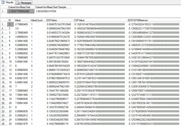
…………I performed queries like the one in Figure 2 against two datasets I’ve used throughout the last two tutorial series, one by on the Duchennes form of muscular dystrophy made publicly available by the Vanderbilt University’s Department of Biostatistics and another on the Higgs Boson provided by the University of California at Irvine’s Machine Learning Repository. Now that I’m familiar with how closely their constituent columns follow the bell curve, I was not surprised to see that the LactateDehydrogenase and PyruvateKinase enzymes scored 0.579157871602764 and 2.25027709042408 respectively, or that the test statistic for the Hemopexin protein was 0.471206505704088. Once again, I can’t guarantee that those figures are accurate in the case of this test, but the values follow the expected order (the same cannot be said of the one-sample Wikipedia version, which varied widely across all of the columns I tested it on). Given that the test statistic is supposed to rise in tandem with the lack of fit, I was likewise not surprised to see that the highly abnormal first float column of the Higgs Boson Dataset scored a 118.555073824395. The second float column obviously follows a bell curve in histograms and had a test statistic of 0.6277795953021942279. Note that the results for the same columns in Goodness-of-Fit Testing with SQL Server Part 7.3: The Anderson-Darling Test were 5.43863473749926, 17.4386371653374, 5.27843535947881, 870424.402686672 and 12987.3380102254 respectively. One of the reasons I posted the code for this week’s test statistic despite by misgivings about its accuracy is that the numbers are easier to read than those for its closest cousin. Unlike the Kolmogorov-Smirnov, Kuiper’s and Lilliefors Tests, the Cramér–von Mises Criterion is not bounded between 0 and 1, but it at least doesn’t reach such inflated sizes as in the Anderson-Darling stat. Furthermore, the vastly higher count in the Higgs Boson Dataset seems to swell the Anderson-Darling results even for clearly Gaussian data like the second float column, which makes it difficult to compare stats across datasets.

Figure 3: Execution Plan for the Cramér–von Mises Criterion (click to enlarge)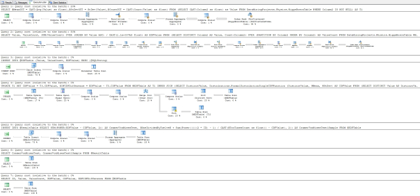

…………Another advantage the Cramér–von Mises Criterion might enjoy over the Anderson-Darling Test is far better performance. The execution plan in Figure 3 is almost identical to those we saw in Goodness-of-Fit Testing with SQL Server Part 7.1: The Kolmogorov-Smirnov and Kuiper’s Tests and Part 7.2: The Lilliefors Test. Once again there are five queries, only two of which have any real cost. Both of those begin with nonclustered Index Seeks, which is usually a good sign. The only really costly savings we might be able to drudge up are with the Hash Match (Aggregate) operator – but there isn’t much point, since the procedure had the same stellar performance as the Kolmogorov-Smirnov, Kuiper’s and Lilliefors Tests. Given that the procedure is structured so similarly to its high-performing kin, it’s not surprising that it took only 24 seconds to race through the 11 million rows in the Higgs Boson Dataset when processing the first float column and 1:15 for the second; in contrast, the Anderson-Darling took a whopping 9:24 for Column1 and 9:09 for Column2. These times will be several orders of magnitude better when run on a real database server instead of my run-down development machine, but it would probably be wise to go with the better-performing measures anyways, assuming they’re otherwise a good fit for our use cases.
…………I originally intended to include the Akaike, Bayesian and several other metrics with “Information Criterion,” in their name, but decided that these measures of mining model fitness would best be handled in an upcoming series titled Information Measurement with SQL Server. The last tutorial series on outlier detection ended with articles on Cook’s Distance and Mahalanobis Distance, which were both intended to segue into that more advanced series (which I’m entirely unqualified to write), in which we’ll tackle various types of entropy, measures of structure, quantification of order and other mind-blowing topics. We’ll hear from such familiar names as Cramér and Kolmogorov again in that series, but first I must take a detour into a topic that could be of immediate benefit to a wide range of SQL Server users. In the upcoming tutorial series Implementing Fuzzy Sets with SQL Server, I’ll explain how the tragically neglected but techniques used in fuzzy sets can be immediately applied to real-world problems that the SQL Server community encounters routinely, particularly those where modeling data on continuous scales would be preferable but is not currently done because of inexact measurement methods. This article was probably the weakest entry in the Goodness-of-Fit series, which was itself only of narrow interest to certain niches in the SQL Server user base; I only went off on this tangent because I recognized my own weaknesses in this area while writing the Outlier Detection with SQL Server series and sought to rectify it through the school of hard knocks. In the future I may tack a few more articles onto the end of this series, such as sample code for Mardia’s Multivariate Skewness and Kurtosis and other multivariate goodness-of-fit tests, but the bulk of this series is complete. In my next post I’ll introduce some of the basic concepts behind fuzzy sets, before providing code samples that should make this treasure trove of techniques immediately available to a wide range of SQL Server users, in order to solve classes of problems that are not being solved efficiently today. As with much of the research into data mining techniques, the academic study of fuzzy sets is at least two decades ahead of the practice. It’s high time it was brought within reach of non-specialists, many of whom could derive surprising practical benefit from these techniques.

See the Wikipedia webpage “Anderson-Darling Test” at http://en.wikipedia.org/wiki/Anderson%E2%80%93Darling_test

[ii] IBID.

[iii] See the comment “Several goodness-of-fit tests, such as the Anderson-Darling test and the Cramer Von-Mises test, are refinements of the K-S test,” at National Institute for Standards and Technology, 2014,  “1.3.5.16 Kolmogorov-Smirnov Goodness-of-Fit Test,” published in the online edition of the Engineering Statistics Handbook. Available at http://www.itl.nist.gov/div898/handbook/eda/section3/eda35g.htm

[iv] See the Wikipedia page “Cramér–von Mises Criterion” at http://en.wikipedia.org/wiki/Cram%C3%A9r%E2%80%93von_Mises_criterion

[v] I derived the formula from Anderson, T.W. and Stephens, M.A., 1994, The Modified Cramer-Von Mises Goodness-of-Fit Criterion for Time Series. Technical Report No. 47, Jan. 17, 1994. Published by the Office of Naval Research and the National Science Foundation. Available at the DTIC Online web address http://www.dtic.mil/dtic/tr/fulltext/u2/a275377.pdf Also see Xiao, Yuanhui; Gordon, Alexander and Yakovlev, Andrei, 2006, “A C++ Program for the Cramér-Von Mises Two-Sample Test,” pp. 1-15 in Journal of Statistical Software, January 2007. Vol. 17, No. 8. Available online at http://www.jourlib.org/paper/2885039#.VIXYZP4o4uU All three authors taught at the University of Rochester, which is on the other side of the city from me. I had to dust off my C++ for this one, which brought back interesting memories of typing “Hello World” while precariously balancing a laptop on my knees at my sister’s house ages ago, after having a few beers and a whole box of chocolates on Valentine’s Day.

[vi] See the Wikipedia page “Cramér–von Mises Criterion” at https://en.wikipedia.org/wiki/Cram%C3%A9r%E2%80%93von_Mises_criterion

[vii] p. 57 , Watson, G. S., 1962, “Goodness-of-Fit Tests on a Circle,” p. 57 in Biometrika, Vol. 49, No. 1 and 2. Available online at http://phdtree.org/pdf/33054228-goodness-of-fit-tests-on-a-circle-ii/

[viii] IBID.