By Steve Bolton

…………As mentioned in previous installments of this series of amateur self-tutorials, goodness-of-fit tests can be differentiated in many ways, including by the data and content types of the inputs and the mathematical properties, data types and cardinality of the outputs, not to mention the performance impact of the internal calculations in between them. Their uses can be further differentiated by the types of probability distributions or regression models they can be applied to and the points within those distributions where their statistical power is highest, such as in the tails of a bell curve or the central point around the median or mean. The Anderson-Darling Test differs from the Kolmogorov-Smirnov Test we recently surveyed and others in its class in a plethora of ways, some of which I was able to glean from sundry comments scattered across the Internet. Unlike many other such tests, it can be applied beyond the usual Gaussian or “normal” distribution to other distributions including the “lognormal, exponential, Weibull, logistic, extreme value type 1” and “Pareto, and logistic.”[1] This is perhaps its major drawing card, since many other such tests are limited to a really narrow range of distributions, usually revolving around the Gaussian.
…………In terms of interpretation of the test statistic, it is “generally valid to compare AD values between distributions and go with the lowest.”[2] When used with the normal distribution it is also “close to optimal” in terms of the Bahadur Slope, one of several methods of assessing the usefulness of the tests statistics produced by goodness-of-fit tests.[3] One of the drawbacks is that “it performs poorly if there are many ties in the data.”[4] Another is that it may be necessary to multiply the final test statistic by specific constants when testing distributions other than the normal[5], but I was unable to find references to any of them in time to include them in this week’s T-SQL stored procedure. This is not true of the Kolmogorov-Smirnov Test we surveyed a few weeks back, which is “distribution-free as the critical values do not depend on whether Gaussianity is being tested or some other form.”[6]

Parameter Estimation and EDA

                This particular limitation is not as much of an issue in the kind of exploratory data mining that the SQL Server community is more likely to use these tests for, given that we’re normally not performing hypothesis testing; I’ve generally shied away from that topic in this series for many reasons that I’ve belabored in previous articles, like the ease of misinterpretation of confidence intervals and the information loss involved in either-or hypothesis rejections. Don’t get me wrong, hypothesis testing is a valuable and often necessary step when trying to prove a specific point, at the stage of Confirmatory Data Analysis (CDA), but most of our mining use cases revolve around informal Exploratory Data Analysis (EDA), a distinction made in the ‘70s by John W. Tukey, the father of modern data mining.[7] Another issue with hypothesis testing is the fact that most of the lookup tables and approximations weren’t designed with datasets consisting of millions of rows, as DBAs and miners of SQL Server cubes encounter every day.

This size difference has a side benefit, in that we generally don’t have to estimate the means and variances of our datasets, which is a much bigger issue in the kinds of small random samples that hypothesis tests are normally applied to. One of the properties of the Anderson-Darling Test is that parameter estimation is less of an issue with it, whereas the Lilliefors Test, the subject of last week’s article, is designed specifically for cases where the variance is unknown. There are apparently special formulations where different combinations of the mean and standard deviation are unknown, but these aren’t going to be common in our use cases, since the mean and variance are usually trivial to compute in an instant for millions of rows. Another noteworthy property that may be of more use to us is the fact that the Anderson-Darling Test is more sensitive to departures from normality in the tails of distributions in comparison with other popular fitness tests.[8]

The Perils and Pitfalls of Equation Translation

                It is not surprising that this long and varied list of properties differentiates the Anderson-Darling Test from the Kolmogorov-Smirnov, Kuiper’s and Lilliefors Tests we’ve surveyed in the last few articles, given that there are some marked differences in its internal calculations. The inner workings apparently involve transforming the inputs into a uniform distribution, which is still a bit above my head, because I’m still learning stats and stochastics as I go. The same can be said of some of the equations I had to translate for this week’s article, which contained some major stumbling blocks I wasn’t expecting. Once of these was the fact that the Anderson-Darling Test is usually categorized along with other methods based on the empirical distribution function (EDF), which as explained in recent articles, involves computing the difference between the actual values and the probabilities generated for them by the distribution’s cumulative distribution function (CDF). Nevertheless, the CDF is used twice in the calculation of the test statistic and the EDF is not used at all, which led to quite a bit of confusion on my part.
…………Another issue I ran into is the fact that the term “N +1 – I” in the formula actually requires the calculation of an order statistic of the kind we used in Goodness-of-Fit Testing with SQL Server, part 6.1: The Shapiro-Wilk Test. I won’t recap that topic here, except to say that it is akin to writing all of the values in a dataset on a sheet of paper in order, then folding it in half and adding them up on each side. Prior to that discovery I was mired in trying various combinations of Lead and Lag that just weren’t returning the right outputs. I found an offhand remark after the fact in an academic paper (which I can’t recall in order to give proper credit) to the effect that the identification of this term as an order statistic is missing from most of the literature on the subject for some unknown reason. As I’ve learned over the past few months, the translation of equations[9] is not always as straightforward as I originally thought it would be (even though I already had some experience doing back in fourth and fifth grade, when my father taught  college physics classes and I used to read all of his textbooks). Other remaining issues with the code in Figure 1 include the fact that I may be setting the wrong defaults for the LOG operations on the CDFValues when they’re equal to zero and the manner in which I handle ties in the order statistics, which may be incorrect. Some of the literature also refers to plugging the standard normal distribution values of 0 and 1 for the mean and standard deviation. Nevertheless, I verified the output of the procedure on two different sets of examples I found on the Internet, so the code may be correct as is.[10]

Figure 1: T-SQL Code for the Anderson-Darling Procedure
CREATE PROCEDURE Calculations.GoodnessofFitAndersonDarlingTestSP
@Database1 as nvarchar(128) = NULL, @Schema1 as nvarchar(128), @Table1 as nvarchar(128),@Column1 AS nvarchar(128)
AS

DECLARE @SchemaAndTable1 nvarchar(400),@SQLString nvarchar(max)
SET @SchemaAndTable1 = @Database1 + ‘.’ + @Schema1 + ‘.’ + @Table1

DECLARE @Mean float,
@StDev float,
@Count  float

DECLARE @ValueTable table
(Value  float)

DECLARE @CDFTable table
(ID bigint IDENTITY (1,1),
Value  float,
CDFValue  float)

DECLARE @ExecSQLString nvarchar(max), @MeanOUT nvarchar(200),@StDevOUT nvarchar(200),@CountOUT nvarchar(200), @ParameterDefinition nvarchar(max)
SET @ParameterDefinition = ‘@MeanOUT nvarchar(200) OUTPUT,@StDevOUT nvarchar(200) OUTPUT,@CountOUT nvarchar(200) OUTPUT ‘
SET @ExecSQLString = ‘SELECT @MeanOUT = CAST(Avg(‘ + @Column1 + ‘) as float),@StDevOUT = CAST(StDev(‘ + @Column1 + ‘)as float),@CountOUT = CAST(Count(‘ + @Column1 + ‘)as float)
       FROM ‘ + @SchemaAndTable1 + ‘
       WHERE ‘ + @Column1 + ‘ IS NOT NULL’

EXEC sp_executesql @ExecSQLString,@ParameterDefinition, @MeanOUT = @Mean OUTPUT,@StDevOUT = @StDev OUTPUT,@CountOUT = @Count OUTPUT

SET @SQLString = ‘SELECT ‘ + @Column1 + ‘ AS Value
FROM ‘ + @SchemaAndTable1 + ‘
WHERE ‘ + @Column1 + ‘ IS NOT NULL’

INSERT INTO @ValueTable
(Value)
EXEC (@SQLString)  

INSERT INTO @CDFTable
(Value, CDFValue)
SELECT T1.Value, CDFValue
FROM @ValueTable AS T1
INNER JOIN  (SELECT DistinctValue, Calculations.NormalDistributionSingleCDFFunction (DistinctValue, @Mean, @StDev) AS CDFValue
       FROM (SELECT DISTINCT Value AS DistinctValue
       FROM @ValueTable) AS T2) AS T3
       ON T1.Value = T3.DistinctValue

SELECT SUM(((1 – (ID * 2)) / @Count) * (AscendingValue + DescendingValue)) – @Count AS AndersonDarlingTestStatistic
FROM (SELECT TOP 9999999999 ID, CASE WHEN CDFValue = 0 THEN 0 ELSE Log(CDFValue) END AS AscendingValue
FROM @CDFTable
ORDER BY ID) AS T1
       INNER JOIN (SELECT ROW_NUMBER() OVER (ORDER BY CDFValue DESC) AS RN, CASE WHEN 1 – CDFValue = 0 THEN 0 ELSE  Log(1 – CDFValue) END AS DescendingValue
       FROM @CDFTable) AS T2
       ON T1.ID = T2.RN

— this statement is included merely for convenience and can be eliminated
SELECT Value, CDFValue
FROM @CDFTable
ORDER BY Value

…………The code turned out to be quite short in comparison to the length of time it took to write and the number of mistakes I made along the way. Most of it self-explanatory for readers who are used to the format of the T-SQL procedures I’ve posted in the last two tutorial series. As usual, there is no null-handling, SQL injection or validation code, nor can the parameters handle brackets, which I don’t allow in my own code. The first four allow users to run the procedure on any column in any database they have sufficient access to. The final statement returns the table of CDF values used to calculate the test statistic, since there’s no reason not to now that the costs have already been incurred; as noted above, “this statement is included merely for convenience and can be eliminated.” The joins in the INSERT statement lengthen the code but actually make it more efficient, by enabling the calculation of CDF values just once for each unique column value. The Calculations.NormalDistributionSingleCDFFunction has been introduced in several previous articles, so I won’t rehash it here. In the SELECT where the test statistic is derived, I used an identity value in the join because the ROW_NUMBER operations can be expensive on big table, so I wanted to avoid doing two in one statement.

Figure 2: Sample Results from the Anderson-Darling Test
EXEC   Calculations.GoodnessofFitAndersonDarlingTestSP
              @Database1 = N’DataMiningProjects’,
              @Schema1 = N’Health’,
              @Table1 = N’DuchennesTable’,
              @Column1 = N’PyruvateKinase’

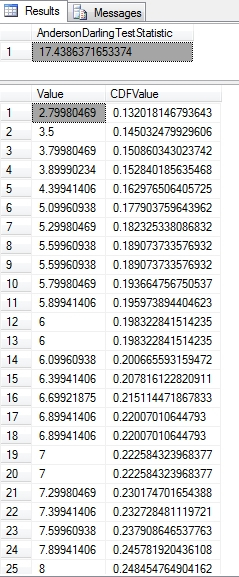
…………One of the concerns I had when running queries like the one in Figure 2 against the 209 rows of the Duchennes muscular dystrophy dataset and the 11 million rows of the Higgs Boson dataset (which I downloaded from the Vanderbilt University’s Department of Biostatistics and University of California at Irvine’s Machine Learning Repository and converted into SQL Server tables for use in these tutorial series) is that the values seemed to be influenced by the value ranges and cardinality of the inputs. Unlike the last three tests covered in this series, it is not supposed to be bounded between 0 and 1. As I discovered when verifying the procedure against other people’s examples, it’s not uncommon for the test statistic to get into the single or double digits. In the examples at the NIST webpage, those for the Lognormal and Cauchy distributions were in the double and triple digits respectively, while that of the double exponential distribution were well above 1, so it may not be unusual to get a test statistic this high. It is definitely not bounded between 0 and 1 like the stats returned by other goodness-of-fit tests, but the range might be distribution-dependent. This is exactly what happened with the LactateDehydrogenase, PyruvateKinase and Hemopexin columns, which scored 5.43863473749926, 17.4386371653374 and 5.27843535947881respectively. Now contrast that range with the Higgs Boson results, where the second float column scored a 12987.3380102254 and the first a whopping 870424.402686672. The problem is not with the accuracy of the results, which are about what I’d expect, given that Column2 clearly follows a bell curve in a histogram while Column1 is ridiculously lopsided. The issue is that for very large counts, the test statistic seems to be inflated, so that it can’t be compared across datasets. Furthermore, once a measure gets up to about six or seven digits to the left of the decimal point, it is common for readers to semiconsciously count the digits and interpolate commas, which is a very slow and tedious process. The test statistics are accurate, but suffer from legibility and comparability issues when using Big Data-sized record counts.

Figure 3: Execution Plan for the Anderson-Darling Procedure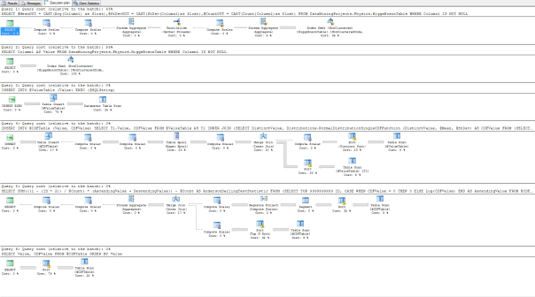

…………The procedure also performed poorly on the super-sized Higgs Boson dataset, clocking in at 9:24 for Column1 and 9:09 for Column2; moreover, it gobbled up several gigs of RAM and a lot of space in TempDB, probably as a result of the Table Spool in the execution plan above. Perhaps some optimization could also be performed on the Merge Join, which was accompanied by some expensive Sort operators, by forcing a Hash Match or Nested Loops. The major stumbling block is the number of Table Scans, which I tried to overcome with a series of clustered and non-clustered indexes on the table variables, but this unexpectedly degraded the execution time badly, in tandem with outrageous transaction log growth. I’m sure a T-SQL expert could spot ways to optimize this procedure, but as it stands, the inferior performance means it’s not a good fit for our use cases, unless we’re dealing with small recordsets and need to leverage its specific properties. All told, the Anderson-Darling procedure has some limitations that make it a less attractive option for general-purpose fitness testing than the Kolmogorov-Smirnov Test, at least for our unique uses cases. On the other hand, it has a well-defined set of uses cases based on a well-established properties, which means it could be applied to a wide variety of niche cases. Among these properties is its superior ability “for detecting most departures from normality.”[11] In the last installment of this series, we’ll discuss the Cramér–von Mises Criterion, another EDF-based method that is closely related to the Anderson-Darling Test and enjoys comparable statistical power in detecting non-normality.[12]

[1] See National Institute for Standards and Technology, 2014,  “1.3.5.14 Anderson-Darling Test,” published in the online edition of the Engineering Statistics Handbook. Available at http://www.itl.nist.gov/div898/handbook/eda/section3/eda35e.htm

[2] Frost, Jim, 2012, “How to Identify the Distribution of Your Data using Minitab,” published March, 2012 at The Minitab Blog  web address http://blog.minitab.com/blog/adventures-in-statistics/how-to-identify-the-distribution-of-your-data-using-minitab

[3] p. 52, No author listed, 1997, Encyclopaedia of Mathematics, Supplemental Vol. 1. Reidel: Dordrecht. This particular page was retrieved from Google Books.

[4] No author listed, 2014, “Checking Gaussianity,” published online at the MedicalBiostatistics.com web address http://www.medicalbiostatistics.com/checkinggaussianity.pdf

[5] See the Wikipedia webpage “Anderson-Darling Test” at http://en.wikipedia.org/wiki/Anderson%E2%80%93Darling_test

[6] See the aforementioned MedicalBiostatistics.com article.

[7] See Tukey, John W., 1977, Exploratory Data Analysis. Addison-Wesley: Reading, Mass. I’ve merely heard about the book second-hand and have yet to read it, although I may have encountered a few sections here and there.

[8] IBID.

[9] For the most part, I depended on the more legible version in National Institute for Standards and Technology, 2014,  “1.3.5.14 Anderson-Darling Test,” published in the online edition of the Engineering Statistics Handbook. Available at http://www.itl.nist.gov/div898/handbook/eda/section3/eda35e.htm All of the sources I consulted though had the same notation, without using the term order statistic.

[10] See Frost, 2012, for the sample data he calculated in Minitab and See Alion System Reliability Center, 2014, “Anderson-Darling: A Goodness of Fit Test for Small Samples Assumptions,” published in Selected Topics in Assurance Related Technologies, Vol. 10, No. 5. Available online at the Alion System Reliability Center web address http://src.alionscience.com/pdf/A_DTest.pdf  These START publications are well-written , so I’m glad I discovered them recently through Freebird2008’s post on Sept. 4, 2008 at the TalkStats thread “The Anderson-Darling Test,” which is available at http://www.talkstats.com/showthread.php/5484-The-Anderson-Darling-Test

[11] See the Wikipedia webpage “Anderson-Darling Test” at http://en.wikipedia.org/wiki/Anderson%E2%80%93Darling_test

[12] IBID.