By Steve Bolton

…………Since I’m teaching myself as I go in this series of self-tutorials, I often have only a vague idea of the challenges that will arise when trying to implement the next goodness-of-fit test with SQL Server. In retrospect, had I known that the Lilliefors Test was so similar to the Kolmogorov-Smirnov and Kuiper’s Tests, I probably would have combined them into single article. The code for this week’s T-SQL stored procedure is nearly the same, as is the execution plan and the performance. The results are also quite similar right to those of the Kolmogorov-Smirnov Test for some of the practice data I’ve used throughout the series, differing in some cases by just a few decimal places. The slight differences may arise from one of the characteristics of the Lilliefors Test that differentiate it from its more famous cousin, namely that “this test of normality is more powerful than others procedures for a wide range of nonnormal conditions.” Otherwise, they share many mathematical properties in common, like location and scale invariance – i.e., the proportions of the test statistics aren’t altered when using a different starting point or multiplying by a common factor.
…………On the other hand, the test is apparently more restrictive than the Kolmogorov-Smirnov, in that I’ve seen it referred to specifically as a normality test and I haven’t encountered any mention of it being applied to other distributions. Furthermore, its primary use cases seems to be those in which the variance of the data is unknown[ii], which often doesn’t apply in the types of million-row tables the SQL Server community works with daily. The late Hubert Lilliefors (1928-2008), a stats professor at George Washington University, published it in a Journal of the American Statistical Association titled “On the Kolmogorov-Smirnov Test for Normality with Mean and Variance Unknown” back in 1967[iii] – so augmenting its more famous cousin in a few niche scenarios seems to have been the raison d’etre from the beginning. We can always use more statistical tests in our toolbox to meet the never-ending welter of distributions that arise from actual physical processes, but I won’t dwell on the Lilliefors Test for long because its narrower use cases are less suited to our needs than those of the broader Kolmogorov-Smirnov Test.

Differences from the Kolmogorov-Smirnov

                Another reason for not dwelling on it for too long is that most of the code is identical to that of the stored procedure posted in last week’s article. The Lilliefors Test quantifies the difference between the empirical distribution function (EDF) and cumulative distribution function (CDF) exactly the same as the Kolmogorov-Smirnov and Kuiper’s Tests do; in plain English, it orders the actual values and ranks them on a scale of 0 to 1 and computes the difference from the theoretical probability for the Gaussian “normal” distribution, or bell curve, which is also ranked on a scale of 0 to 1. A couple of notes of caution are in order here, because some of the sources I consulted mentioned inputting Z-Scores into the formula and using the standard normal distribution rather than the actual mean and standard deviation of the dataset, but I verified that the procedure is correct as it stands now against an example at Statd.com.[iv]
…………One of the main characteristics that set it apart from the Kolmogorov-Smirnov Test is that the test statistic is compared against the Lilliefors distribution, which apparently has a better Bahadur Slope[v] (one of many measures of the efficiency of test statistics) than its competitors in certain hypothesis testing scenarios. That is a broad topic I’ve downplayed for several reasons throughout the last two tutorial series. Among the reasons I’ve brought up in the past are the fact that SQL Server users more likely to be using these tests for exploratory data mining, not proving specific points of evidence, as well as the ease of misinterpretation of p-values, critical values and confidence intervals even among professional academic researchers. What we need are continuous measures of how closely a dataset follows a particular distribution, not simple Boolean either-or choices of the kind used in hypothesis testing, which reduce the information content of the test statistics as sharply as casting a float data type to a bit would in T-SQL. Furthermore, many of the lookup tables and approximation used in hypothesis testing are only valid up to a few hundred values, not the several million that we would need in Big Data scenarios.

Abde and Molin’s Approximation

                The Lilliefors distribution was originally derived from Monte Carlo simulations (a broad term encompassing many types of randomized trials) and at least one attempt has been made to approximate it through a set of constants and equations.[vi] I implemented the approximation developed by Hervé Abdi and Paul Molin, but the first couple of SELECTs and the declarations following the comment “code for Molin and Abdi’s approximation” can be safely deleted if you don’t have a need for the P-values the block generates. I verified the P-Values and @A constants used to generate it against the examples given in their undated manuscript “Lilliefors/Van Soest’s Test of Normality,” but as is commonly the case with such workarounds in hypothesis testing, the algorithm is inapplicable when Big Data-sized values and counts are plugged into it.
…………Once @A falls below about 0.74 the approximation begins to return negative P-values and when it climbs above about 5.66 it produces P-values greater than 1, which I believe are invalid under the tenets of probability theory. Most of the practice datasets I plugged into the approximation returned invalid outputs, most of them strongly negative. This is a problem I’ve seen with other approximation techniques when they’re fed values beyond the expected ranges. Nevertheless, since I already coded it, I’ll leave that section intact in case anyone runs into scenarios where they can apply it to smaller datasets.

Figure 1: T-SQL Code for the Lilliefors Goodness-of-Fit Test
CREATE PROCEDURE [Calculations].[GoodnessOfFitLillieforsTest]
@Database1 as nvarchar(128) = NULL, @Schema1 as nvarchar(128), @Table1 as nvarchar(128),@Column1 AS nvarchar(128), @OrderByCode as tinyint
AS

DECLARE @SchemaAndTable1 nvarchar(400),@SQLString nvarchar(max)
SET @SchemaAndTable1 = @Database1 + ‘.’ + @Schema1 + ‘.’ + @Table1

DECLARE @Mean float,
@StDev float,
@Count  float

DECLARE @EDFTable table
(ID bigint IDENTITY (1,1),
Value float,
ValueCount bigint,
EDFValue float,
CDFValue decimal(38,37),
EDFCDFDifference decimal(38,37)) 

DECLARE @ExecSQLString nvarchar(max), @MeanOUT nvarchar(200),@StDevOUT nvarchar(200),@CountOUT nvarchar(200), @ParameterDefinition nvarchar(max)
SET @ParameterDefinition = ‘@MeanOUT nvarchar(200) UTPUT,@StDevOUT nvarchar(200) OUTPUT,@CountOUT nvarchar(200) OUTPUT ‘
SET @ExecSQLString = ‘SELECT @MeanOUT = CAST(Avg(‘ + @Column1 + ‘) as float),CAST(@StDevOUT = StDev(‘ + @Column1 + ‘) as float),CAST(@CountOUT = Count(‘ + @Column1 + ‘) as float)
       FROM ‘ + @SchemaAndTable1 + ‘
       WHERE ‘ + @Column1 + ‘ IS NOT NULL’

EXEC sp_executesql @ExecSQLString,@ParameterDefinition, @MeanOUT = @Mean OUTPUT,@StDevOUT = @StDev OUTPUT,@CountOUT = @Count OUTPUT

SET @SQLString = ‘SELECT Value, ValueCount, SUM(ValueCount) OVER (ORDER BY Value ASC) / CAST(‘ + CAST(@Count as nvarchar(50)) + ‘AS float) AS EDFValue
       FROM (SELECT DISTINCT  ‘ + @Column1 + ‘ AS      Value, Count(‘ + @Column1 + ‘) OVER (PARTITION BY ‘ + @Column1 + ‘ ORDER BY ‘ + @Column1 + ‘) AS ValueCount
              FROM ‘ + @SchemaAndTable1 + ‘
WHERE ‘ + @Column1 + ‘ IS NOT NULL) AS T1‘              

INSERT INTO @EDFTable (Value, ValueCount, EDFValue)
EXEC (@SQLString)

UPDATE T1
SET CDFValue = T3.CDFValue, EDFCDFDifference = EDFValue – T3.CDFValue
FROM @EDFTable AS T1
       INNER JOIN (SELECT DistinctValue, Calculations.NormalCalculationsingleCDFFunction (DistinctValue, @Mean, @StDev) AS CDFValue
       FROM (SELECT DISTINCT Value AS DistinctValue
              FROM @EDFTable) AS T2) AS T3
       ON T1.Value = T3.DistinctValue

DECLARE @b0 float = 0.37872256037043,
@b1 float = 1.30748185078790,
@b2 float = 0.08861783849346,
@A float,
@PValue float,
@LillieforsTestStatistic float 

SELECT @LillieforsTestStatistic = Max(ABS(EDFCDFDifference))
FROM @EDFTable

— code for Molin and Abdis approximation
— =======================================
SELECT @A = ((-1 * (@b1 + @Count)) + Power(Power((@b1 + @Count), 2) – (4 * @b2 * (@b0 – Power(@LillieforsTestStatistic, –2))), 0.5)) / (2 * @b2)
SELECT @PValue = –0.37782822932809 + (1.67819837908004 * @A)
– (3.02959249450445 * Power(@A, 2))
+ (2.80015798142101 * Power(@A, 3))
– (1.39874347510845 * Power(@A, 4))
+ (0.40466213484419 * Power(@A, 5))
– (0.06353440854207 * Power(@A, 6))
+ (0.00287462087623 * Power(@A, 7))
+ (0.00069650013110 * Power(@A, 8))
– (0.00011872227037 * Power(@A, 9))
+ (0.00000575586834 * Power(@A, 10))

SELECT  @LillieforsTestStatistic AS LillieforsTestStatistic, @PValue AS PValueAbdiMollinApproximation
SELECT ID, Value, ValueCount, EDFValue, CDFValue, EDFCDFDifference
FROM @EDFTable
ORDER BY CASE WHEN @OrderByCode = 1 THEN ID END ASC,
CASE WHEN @OrderByCode = 2 THEN ID END DESC,
CASE WHEN @OrderByCode = 3 THEN Value END ASC,
CASE WHEN @OrderByCode = 4 THEN Value END DESC,
CASE WHEN @OrderByCode = 5 THEN ValueCount END ASC,
CASE WHEN @OrderByCode = 6 THEN ValueCount END DESC,
CASE WHEN @OrderByCode = 7 THEN EDFValue END ASC,
CASE WHEN @OrderByCode = 8 THEN EDFValue END DESC,
CASE WHEN @OrderByCode = 9 THEN CDFValue END ASC,
CASE WHEN @OrderByCode = 10 THEN CDFValue END DESC,
CASE WHEN @OrderByCode = 11 THEN EDFCDFDifference END ASC,
CASE WHEN @OrderByCode = 12 THEN EDFCDFDifference END DESC

Figure 2: Sample Results from the Lilliefors Goodness-of-Fit Test
EXEC   Calculations.GoodnessofFitLillieforsTestSP
              @DatabaseName = N’DataMiningProjects‘,
              @SchemaName = N’Health‘,
              @TableName = N’DuchennesTable‘,
             @ColumnName = N’LactateDehydrogenase‘,
              @OrderByCode = ‘1’

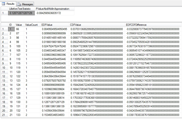
…………Aside from the approximation section, the code in Figure 1 is almost identical to that of last week’s procedure, so I won’t belabor the point by rehashing the explanation here. As usual, I used queries like the one in Figure 2 to test the procedure against several columns in a 209-row dataset on the Duchennes form of muscular dystrophy and an 11-million-row dataset on the Higgs Boson, which are made publicly available by the Vanderbilt University’s Department of Biostatistics and University of California at Irvine’s Machine Learning Repository respectively. It is not surprising that the results nearly matched the Kolmogorov-Smirnov test statistic for many practice columns. For example, the LactateDehydrogenase enzyme scored 0.128712871287129 here and  0.131875117324784 on the Kolmogorov-Smirnov, while the less abnormal Hemopexin protein scored 0.116783569553499 on the Lilliefors and 0.0607407215998911on the Kolmogorov-Smirnov Test. Likewise, the highly abnormal first float column and Gaussian second column in the Higgs Boson table had test statistics of 0.276267238731715 and 0.0181893798916693 respectively, which were quite close to the results of the Kolmogorov-Smirnov. I cannot say if the departure in the case of Hemopexin was the result of some property of the test itself, like its aforementioned higher statistical power for detecting non-normality, or perhaps a coding error on my part. If so, then it would probably be worth it to calculate the Lilliefors test statistic together with the Kolmogorov-Smirnov and Kuiper’s measures and return them in one batch, to give end users a sharper picture of their data at virtually no computational cost.

Figure 3: Execution Plan for the Lilliefors Goodness-of-Fit Test (click to enlarge)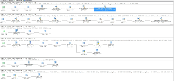

…………There were six queries in the execution plan, just as there were for last week’s tests, but the first accounted for 19 percent and the second 82 percent of the batch total. Both of those began with non-clustered Index Seeks, which is exactly what we want to see. Only the second would provide any worthwhile opportunities for further optimization, perhaps by targeting the only three operators besides the seek that contributed anything worthwhile to the query cost: a Hash Match (Aggregate) at 14 percent, a Stream Aggregate that accounted for 10 percent and two Parallelism (Repartition Streams) that together amount to 53 percent . Optimization might not really be necessary, given that the first float column in the mammoth Higgs Boson dataset returned in just 23 seconds and the second in 27. Your marks are likely to be several orders of magnitude better, considering that the procedure was executed on an antiquated semblance of a workstation that is an adventure to start up, not a real database server. The only other fitness tests in this series this fast were the Kolmogorov-Smirnov and Kuiper’s Tests, which I would have calculated together with this test in a single procedure if I’d known there was so much overlap between them. The Anderson-Darling Test we’ll survey in the next installment of the series is also included in the same category of EDF-based fitness tests, but has less in common with the Lilliefors Test and its aforementioned cousins. Unfortunately, high performance is apparently not among the characteristics the Anderson-Darling Test shares with its fellow EDF-based methods. That’s something of a shame, since it is more widely by real statisticians than many other goodness-of-fit tests.

p. 1, Abdi, Hervé and Molin, Paul, undated manuscript “Lilliefors/Van Soest’s Test of Normality,” published at the University of Texas at Dallas School of Behavioral and Brain Sciences web address https://www.utdallas.edu/~herve/Abdi-Lillie2007-pretty.pdf

[ii] See the Wikipedia page “Lilliefors Test” at http://en.wikipedia.org/wiki/Lilliefors_test

[iii] Lilliefors, Hubert W., 1967, “On the Kolmogorov-Smirnov Test for Normality with Mean and Variance Unknown,” pp. 399-402 in Journal of the American Statistical Association, Vol. 62, No. 318. June, 1967.

[iv] See the Statd.com webpage “Lilliefors Normality Test” at http://statltd.com/articles/lilliefors.htm

[v] See Arcones, Miguel A., 2006, “On the Bahadur Slope of the Lilliefors and the Cramér–von Mises Tests of Normality,” pp. 196-206 in the Institute of Mathematical Statistics Lecture Notes – Monograph Series. No. 51. Available at the web address https://projecteuclid.org/euclid.lnms/1196284113

[vi] See p. 3, Abdi and Molin and the aforementioned Wikipedia page “Lilliefors Test” at http://en.wikipedia.org/wiki/Lilliefors_test