By Steve Bolton

…………In the last installment of this amateur series of self-tutorials, we saw how the Shapiro-Wilk Test might probably prove less useful to SQL Server users, despite the fact that it is one of the most popular goodness-of-fit tests among statisticians and researchers. Its impressive statistical power is rendered impotent by the fact that the logic of its internal calculations limits it to inputs of just 50 rows (or up to 2,000 when certain revisions are applied), which is chump change when we’re talking about SQL Server tables that often number in the millions of rows. Thankfully, a little-known rival in the same category[1] is available that shares few of the drawbacks that make Shapiro-Wilk such a disappointing choice for our particular use cases. In fact, the Ryan-Joiner Test “is very highly correlated with that of Shapiro and Wilk, so either test may be used and will produce very similar resultspWhen wading through various head-to-head comparisons of the goodness-of-fit tests published on the Internet, I noticed that on the occasions when the Ryan-Joiner Test was mentioned, it received favorable marks like this review by Jim Colton at the Minitab Blog:

                “I should note that the three scenarios evaluated in this blog are not designed to assess the validity of the Normality assumption for tests that benefit from the Central Limit Theorem, such as such as 1-sample, 2-sample, and paired t-tests. Our focus here is detecting Non-Normality when using a distribution to estimate the probability of manufacturing defective (out-of-spec) unit.
…………“In scenario 1, the Ryan-Joiner test was a clear winner. The simulation results are below…
…………“…The Anderson-Darling test was never the worst test, but it was not nearly as effective as the RJ test at detecting a 4-sigma outlier. If you’re analyzing data from a manufacturing process tends to produce individual outliers, the Ryan-Joiner test is the most appropriate…”
…………“…The RJ test performed very well in two of the scenarios, but was poor at detecting Non-Normality when there was a shift in the data. If you’re analyzing data from a manufacturing process that tends to shift due to unexpected changes, the AD test is the most appropriate.”[3]

…………The most striking drawback is the paucity of public information available on the test, which doesn’t even have a Wikipedia page, thereby forcing me to resort to even less professional sources like Answers.com for matter-of-fact explanations like this: “The Ryan-Joiner test is implemented in the Minitab software package but not widely elsewhere.”[4] It was apparently the brainchild of Brian Joiner and Barbara Ryan, “the founder of Minitab,” but I was unable to find a publicly available copy of the original academic paper they published on the test back in 1976 until after I’d already written most of the code below.[5] Publication of this kind signifies that it is not a proprietary algorithm exclusively owned by Minitab, so we are free to implement it ourselves – provided we can find adequate detail on its inner workings, which turned out to be a tall order. The main drawback of the Ryan-Joiner Test is the difficulty in finding information that can be applied to implementation and testing, which is certainly a consequence of its close association with Minitab, a stats package that competes only tangentially with SQL Server Data Mining (SSDM) as I addressed in Integrating Other Data Mining Tools with SQL Server, Part 2.1: The Minuscule Hassles of Minitab and Integrating Other Data Mining Tools with SQL Server, Part 2.2: Minitab vs. SSDM and Reporting Services. This makes it somewhat opaque, but it I was able to overcome this inscrutability enough to get a T-SQL version of it up and running.
…………The underlying mechanisms are still somewhat unclear, but this brief introduction in the LinkedIn discussion group Lean Sigma Six Group Brazil is adequate enough for our purposes:  “This test assesses normality by calculating the correlation between your data and the normal scores of your data. If the correlation coefficient is near 1, the population is likely to be normal. The Ryan-Joiner statistic assesses the strength of this correlation; if it falls below the appropriate critical value, you will reject the null hypothesis of population normality.”[6] As usual, I’ll be omitting those critical values, because of the numerous issues with hypothesis testing I’ve pointed out in previous blog posts. Apparently my misgivings are widely shared by professional statisticians and mathematicians who actually know what they’re talking about, particularly when it comes to the ease and frequency with which all of the caveats and context that statements of statistical significance are carelessly dispensed with. It is not that significance level stats aren’t useful, but that the either-or nature of standard hypothesis testing techniques discards an awful lot of information by effectively shrinking our hard-won calculations down to simple Boolean either-or choices; not only is this equivalent to casting a float or decimal value down to a SQL Server bit data type, but can also easily lead to errors in interpretation. For this reason and concerns about brevity and simplicity, I’ll leave out the critical values, which can be easily tacked on to my code by anyone with a need for them.

Interpreting the Results in Terms of the Bell Curve

                Aside from that, the final test statistic isn’t that hard to interpret: the closer we get to 1, the more closely the data follows the Gaussian or “normal” distribution, i.e. the bell curve. So far, my test results have all remained within the range of 0 to 1 as expected, but I cannot rule out the possibility that in some situations an undiscovered error will cause them to exceed these bounds. When writing the T-SQL code in Figure 1 I had to make use of just two incomplete sources[7], before finally finding the original paper by Ryan and Joiner at the Minitab website late in the game.[8] This find was invaluable because it pointed out that the Z-Scores (a basic topic I explained way back in Outlier Detection with SQL Server, part 2.1: Z-Scores) in the internal calculations should be done against the standard normal distribution, not the data points.
…………My standard disclaimer that I still a novice in the fields of data mining and statistics and that my sample code has not yet been thoroughly tested ought not be glossed over, given the number of other mistakes I caught myself making when writing the code below. At one point I accidentally used a minus sign rather than an asterisk in the top divisor; I tested it once against the wrong online calculator, for the normal probability density function (PDF) rather than the cumulative density function (CDF); later, I realized I should have used the standard normal inverse CDF rather than the CDF or PDF; I also used several different improper step values for the RangeCTE, including one that was based on minimum and maximum values rather than the count and another based on fractions. Worst of all, I garbled my code at the last minute by accidentally (and not for the first time) using the All Open Documents option with Quick Replace in SQL Server Management Studio (SSMS). Once I figured out my mistakes, the procedure ended up being a lot shorter and easier to follow than I ever expected. Keep in mind, however, that I didn’t have any published examples to test it against, so there may be other reliability issues lurking within.

Figure 1: T-SQL Code for the Ryan-Joiner Test Procedure
CREATE PROCEDURE [Calculations].[NormalityTestRyanJoinerTestSP]
@Database1 as nvarchar(128) = NULL, @Schema1 as nvarchar(128), @Table1 as nvarchar(128),@Column1 AS nvarchar(128)
AS

DECLARE @SchemaAndTable1 nvarchar(400),@SQLString nvarchar(max)
SET @SchemaAndTable1 = @Database1 + ‘.’ + @Schema1 + ‘.’ + @Table1

DECLARE @ValueTable table
(ID bigint IDENTITY (1,1),
Value float)

SET @SQLString = ‘SELECT ‘ + @Column1 + ‘ AS Value
FROM ‘ + @SchemaAndTable1 +
‘ WHERE ‘ + @Column1 + ‘ IS NOT NULL’ 

INSERT INTO @ValueTable
(Value)
EXEC (@SQLString)

DECLARE  @Var AS decimal(38,11),
@Count bigint,
@ConstantBasedOnCount decimal(5,4),
@Mean AS decimal(38,11) 

SELECT @Count = Count(*), @Var = Var(Value)
FROM @ValueTable
— the NOT NULL clause is not necessary here because that’s taken care of the in @SQLString 

SELECT @ConstantBasedOnCount = CASE WHEN @Count > 10 THEN 0.5 ELSE 0.375 END

; WITH RangeCTE(RangeNumber) as
(
    SELECT 1 as RangeNumber   

       UNION ALL

    SELECT RangeNumber + 1
        FROM RangeCTE
        WHERE RangeNumber  < @Count
) 

SELECT SUM(Value * RankitApproximation) /  Power((@Var * (@Count – 1)  * SUM(Power(CAST(RankitApproximation AS float), 2))), 0.5) AS RyanJoinerTestStatistic
FROM (SELECT RN, Value, Calculations.NormalDistributionInverseCDFFunction((RN – @ConstantBasedOnCount) / (@Count + 1 – (2 * @ConstantBasedOnCount))) AS RankitApproximation
       FROM (SELECT ROW_NUMBER() OVER (ORDER BY Value) AS RN, Value
              FROM @ValueTable AS T0) AS T1
       INNER JOIN RangeCTE AS T2
       ON  T1.RN = T2.RangeNumber) AS T3
OPTION (MAXRECURSION 0) 

…………Much of the code above is easy to follow if you’ve seen procedures I’ve posted over the last two tutorial series. As usual, the parameters and first couple of lines in the body allow users to perform the test on any column in any database they have sufficient access to, as well as to adjust the precision of the calculations to avoid arithmetic overflows. Starting with my last article, I began using a lot less dynamic SQL to code procedures like these, by instead caching the original values in a @ValueTable table variable. A couple of simple declarations and assignments needed for the rest of the computations follow this. The RangeCTE generates a set of integers that is fed to the Calculations.NormalDistributionInverseCDFFunction I introduced in Goodness-of-Fit Testing with SQL Server, part 2: Implementing Probability Plots in Reporting Services.
…………In lieu of making this article any more verbose and dry than it absolutely has to be, I’ll omit a rehash of that topic and simply point users back to the code from that previous article. Once those numbers are derived, the calculations are actually quite simple in comparison to some of the more complex procedures I’ve posted in the past. As usual, I’ll avoid a precise explanation of how I translated the mathematical formulas into code, for the same reason that driver’s ed classes don’t require a graduate degree in automotive engineering: end users need to be able to interpret the final test statistic accurately – which is why I’m not including the easily misunderstood critical values – but shouldn’t be bothered with the internals. I’ve supplied just enough detail so that the T-SQL equivalent of a mechanic can fix my shoddy engineering, if need be. It may be worth noting though that I can’t simply use the standard deviation in place of the root of the variance as I normally do, because the square root in the Ryan-Joiner equations is calculated after the variance has been multiplied by other terms.

Figure 2: Sample Results from Ryan-Joiner Test Procedure
EXEC   Calculations.NormalityTestRyanJoinerTestSP
              @DatabaseName = N’DataMiningProjects’,
              @SchemaName = N’Health’,
              @TableName = N’DuchennesTable’,
              @ColumnName = N’Hemopexin’

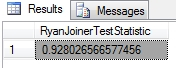
…………The sample query in Figure 2 was run against a column of data on the Hemopexin protein contained within a dataset on the Duchennes form of muscular dystrophy, which I downloaded long ago from the Vanderbilt University’s Department of Biostatistics and converted to a SQL Server table. Since this table only has 209 rows and occupies just 9 kilobytes, I customarily stress test the procedures I post in these tutorials against an 11-million-row table of data on the Higgs Boson, which is made freely available by the University of California at Irvine’s Machine Learning Repository and now occupies nearly 6 gigabytes in the same database.
…………I also tested it against columns in other tables I’m quite familiar with and discovered a pattern that is both comforting and disconcerting at the same time: the test statistic is indeed closer to 0 than 1 on columns I already know to be abnormal, but there may be a scaling issue in the internal calculations because the values are still unexpectedly high for all columns. I know from previous goodness-of-fit and outlier detection tests that the Hemopexin column is more abnormal than some of the other Duchennes columns and as expected, it had a lower Ryan-Joiner statistic; the problem is that it was still fairly close to 1. Likewise, the histograms I posted way back in Outlier Detection with SQL Server, part 6.1: Visual Outlier Detection with Reporting Services clearly show that the first float column in the Higgs Boson dataset is hopelessly lopsided and therefore can’t come from a normal distribution, while the second follows a clear bell curve. It is not surprising then that the former scored a 0.909093348747035 and the latter a 0.996126753961487 in the Ryan-Joiner Test. The order of the values always seems to correctly match the degree of normality for every practice dataset I use, which is a good sign, but the gaps between them may not be proportionally correct. In the absence of example data to verify my procedure against, I can’t tell for sure if this is a problem or not.

Next Up: Kolmogorov and EDF-Based Tests

               Either way, the test is useful as-is, because it at least assigns test statistic values that are in the expected order, regardless of whether or not they are scaled correctly. These results come at a moderate, tolerable performance cost, clocking in at 6:43 for the first float column and 6:14 for the second. As usual, your results will probably be several orders of magnitude better than mine, given that I’m using a clunker of a development machine, not a real database server. The execution plans consist of two queries, the second of which accounts for 97 percent of the cost of the whole batch; out of the 24 operators in that query, a single Sort accounts for 96 percent of the cost. It occurs prior to a Merge Join, so there may be some way to optimize the procedure with join hints or recoding with optimization in mind. We’re unlikely to get much benefit out of analyzing the execution plan further, because it consists almost entirely of spools and Compute Scalar operators with infinitesimal costs, plus two Index Seeks, which is what we want to see.
…………The Ryan-Joiner Test performs well enough that DBA and data miners might find it a more useful addition to their toolbelt than the far better-known Shapiro-Wilk Test, which is simply inapplicable to most Big Data scenarios because of its fatal limitations on input sizes. There may be some lingering concerns about it reliability, but this can be rectified through a more diligent search of the available literature for examples that we can test it against; if we really need this particular statistic, then conferring with a professional statistician for ten minutes to verify the correctness of the results might also get the job done. If misgivings about its reliability are a real concern, then we can always turn to the alternatives we’ll cover in the next segment of this series, like the Kolmogorov-Smirnov (my personal favorite, which was also invented by my favorite mathematician), Anderson-Darling Kuiper’s and Lilliefors Tests, as well as the Cramér–von Mises Criterion. Judging from the fact that experts seem to divide the various goodness-of-fit tests into categories along the same lines[9], I was right to segregate the Jarque-Bera and D’Agostino’s K-Squared Test into a separate segment at the beginning of this series for measures based on kurtosis and skewness. The Shapiro-Wilk and Ryan-Joiner Tests likewise have a separate set of internal mechanism in commons, based on measures of correlation. In the next five articles, we’ll cover a set of goodness-of-fit measures that rely on a different type of internal mechanism, the empirical distribution function (EDF), which is a lot easier to calculate and explain than the long-winded name would suggest.

[1] These authors say it is  “similar to the SW test”:  p. 2142, Yap, B. W. and Sim, C. H., 2011, “Comparisons of Various Types of Normality Tests,” pp. 2141-2155 in Journal of Statistical Computation and Simulation, Vol. 81, No. 12. Also see the remark to the effect that “This test is similar to the Shapiro-Wilk normality test” at Gilberto, S. 2013, “Which Normality Test May I Use?” published in the Lean Sigma Six Group Brazil discussion group, at the LinkedIn web address http://www.linkedin.com/groups/Which-normality-test-may-I-3713927.S.51120536

[2] See the Answers.com webpage “What is Ryan Joiner Test” at http://www.answers.com/Q/What_is_Ryan_joiner_test

[3] Colton, Jim, 2013, “Anderson-Darling, Ryan-Joiner, or Kolmogorov-Smirnov: Which Normality Test Is the Best?” published Oct. 10, 2013 at The Minitab Blog web address http://blog.minitab.com/blog/the-statistical-mentor/anderson-darling-ryan-joiner-or-kolmogorov-smirnov-which-normality-test-is-the-best

[4] See the aforementioned Answers.com webpage.

[5] See the comment by the user named Mikel on Jan. 23, 2008 in the iSixSigma thread “Ryan-Joiner Test” at http://www.isixsigma.com/topic/ryan-joiner-test/

[6] Gilberto, S. 2013, “Which Normality Test May I Use?” published in the Lean Sigma Six Group Brazil discussion group, at the LinkedIn web address http://www.linkedin.com/groups/Which-normality-test-may-I-3713927.S.51120536

[7] No author listed, 2014, “7.5 – Tests for Error Normality,” published at the Penn State University web address https://onlinecourses.science.psu.edu/stat501/node/366 .This source has several other goodness-of-test formulas arranged in a convenient format. Also see Uaieshafizh, 2011, “Normality Test Dengan Menggunakan Uji Ryan-Joiner,” published Nov. 1, 2011 at the Coretan Uaies Hafizh web address http://uaieshafizh.wordpress.com/2011/11/01/uji-ryan-joiner/ . Translated from Indonesian by Google Translate.

[8] Ryan, Jr., Thomas A. and Joiner, Brian L., 1976, “Normal Probability Plots and Tests for Normality,” Technical Report, published by the Pennsylvania State University Statistics Department. Available online at the Minitab web address http://www.minitab.com/uploadedFiles/Content/News/Published_Articles/normal_probability_plots.pdf

[9] For an example, see p. 2143, Yap, B. W. and Sim, C. H., 2011, “Comparisons of Various Types of Normality Tests,” pp. 2141-2155 in Journal of Statistical Computation and Simulation, Vol. 81, No. 12. Available online at the web address http://www.tandfonline.com/doi/pdf/10.1080/00949655.2010.520163 “Normality tests can be classified into tests based on regression and correlation (SW, Shapiro–Francia and Ryan–Joiner tests), CSQ test, empirical distribution test (such as KS, LL, AD andCVM), moment tests (skewness test, kurtosis test, D’Agostino test, JB test), spacings test (Rao’s test, Greenwood test) and other special tests.” I have yet to see the latter two tests mentioned anywhere else, so I’ll omit them from the series for now on the grounds that sufficient information will likely be even harder to find than it was for the Ryan-Joiner Test.