

By Steve Bolton
…………Just as a good garage mechanic will fill his or her Craftsman with tools designed to fix specific problems, it is obviously wise for data miners to stockpile a wide range of algorithms, statistical tools, software packages and the like to deal with a wide variety of user scenarios. Some of the tests and algorithms I’ve covered in this amateur self-tutorial series and the previous one on outlier detection are applicable to a broad range of problems, while others are tailor-made to address specific issues; what works in one instance may be entirely inappropriate in a different context. For example, some fitness tests are specifically applicable only to linear regression and other to logistic regression, as explained in Goodness-of-Fit Testing with SQL Server, part 4.1::R2, RMSE and Regression-Related Routines and Goodness-of-Fit Testing with SQL Server part 4.2:: The Hosmer-Lemeshow Test. Other measures we’ve surveyed recently, like the Chi-Squared, Jarque-Bera and D’Agostino-Pearson Tests, can only be applied to particular probability distributions or are calculated in ways that can be a drag on performance, when run against the wrong type of dataset. The metric I’ll be discussing this week stands out as one of the most popular goodness-of-fit tests, in large part because it is has better “statistical power,” which is a numerical measure of how often the actual effects of a variable are detected by a particular test.
…………The Shapiro-Wilk Test is also apparently flexible enough to be extended to other distribution beyond the “normal” Gaussian (i.e. the bell curve), such as the uniform, the exponential, and to a certain extent “to any symmetric distribution.”[1] Its flexibility is augmented by scale and origin invariance, two properties that statisticians prefer to endow their metrics with because multiplying the terms by a common factor or choosing a different starting point doesn’t lead to incomparable values.[2] For these reasons it is widely implemented in statistical software that competes in a tangential way with SQL Server Data Mining (SSDM), most notably “R, Stata, SPSS and SAS.”[3] As we shall see, however, there is less incentive to implement it in SQL Server than in these dedicated stats packages, because of the specific nature of the datasets we work with.
The Fatal Flaw of Shapiro-Wilk for Big Data
The usefulness of the Shapiro-Wilk Test is severely constrained by a number of drawbacks, such as sensitivity to outliers and the fact that its authors envisioned it as an adjunct to the kind of visualizations we covered in Goodness-of-Fit Testing with SQL Server, part 2: Implementing Probability Plots in Reporting Services, not as a replacement for them.[4] The fatal flaw, however, is that the Shapiro-Wilk Test can only handle datasets up to 50 rows in size; approximations have been developed by statisticians like Patrick Royston that can extend it to at least 2,000 rows, but that is still a drop in the bucket compared to the millions of rows found in SQL Server tables. As I’ve pointed out in previous articles, one of the great strengths of the “Big Data” era is that we can now plumb the depths of such huge treasures troves in order to derive information of greater detail, which is an advantage we shouldn’t have to sacrifice merely to accommodate metrics that were designed generations ago with entirely different contexts in mind. Furthermore, the test is normally used in hypothesis testing on random samples when the means and variances are unknown, which as I have explained in the past, are not user scenarios that the SQL Server community will encounter often.[5] The means and variances of particular columns are trivial to calculate with built-in T-SQL functions. Moreover, random sampling is not as necessary in our field because we have access to such huge repositories of information, which are often equivalent to the full population, depending on what questions we choose to ask about our data.
…………I’ll have to implement the T-SQL code for this article against a small sample of our available practice data, simply because of the built-in limitation on row counts. In order to accommodate larger datasets, we’d have to find a different way of performing the internal calculations, which are subject to combinatorial explosion. The main sticking point it a constant in the Shapiro-Wilk equations which must be derived through covariance matrices, which are too large to calculate for large datasets, regardless of the performance costs. As Royston notes, deriving the constant for a 1,500-row table would require the storage of 1,126,500 reals, given that the covariance matrix requires a number of comparisons equivalent to the count of the table multiplied by one less than itself. That exponential growth isn’t ameliorated much by the fact that those results are then halved; I’m still learning the subject of computational complexity classes so I can’t identify which this calculation might fit into, but it certainly isn’t one of those that are easily computable in polynomial time.
Workarounds for Combinatorial Explosion
My math may be off, but I calculated that stress-testing the Shapiro-Wilk procedure against the first float column in the 11-million-row Higgs Boson Dataset, which I downloaded from the University of California at Irvine’s Machine Learning Repository and converted into a SQL Server table of about 6 gigabytes) would require about 1.2 trillion float values and 67 terabytes of storage space. I have the sneaking suspicion that no one in the SQL Server community has that much free space in their TempDB. And that is before factoring in such further performance hits as the matrix inversion and other such transforms.
…………While writing a recent article on Mahalanobis Distance, combinatorial explosion of matrix determinants forced me to scrap my sample code for a type of covariance matrix that compared the global variance values for each column against one another; even that was a cheap workaround for calculating what amounts to a cross product against each set of local values. In this case, we’re only talking about a bivariate comparison, so inserting the easily calculable global variance value would leave us with a covariance matrix of just one entry, which isn’t going to fly.[6] We can’t fudge the covariance matrix in this way, but it might be possible to use one of Royston’s approximations to derive that pesky constant in a more efficient way. Alas, I was only able to read a couple of pages in his 1991 academic journal article on the topic, since Springer.com charges an arm and a leg for full access. I had the distinct sense, however, that it would still not scale to the size of datasets typically associated with the Big Data buzzword. Furthermore, a lot of it was still over my head, as was the original 1965 paper by Samuel S. Shapiro and Martin B. Wilk (although not as far as such topics used to be, which is precisely why I am using exercises like these in order to acquire the skills I lack). Thankfully, that article in Biometrika provides an easily adaptable table of lookup values for that constant[7], as well as a legible example that I was able to verify my results against. Figure 1 below provides DDL for creating a lookup table to hold those values, which you’ll have to copy yourself from one of the many publicly available sources on the Internet, including the original paper.[8]
Figure 1: DDL for the Shapiro-Wilk Lookup Table
CREATE TABLE [Calculations].[ShapiroWilkLookupTable](
[ID] [smallint] IDENTITY(1,1) NOT NULL,
[ICount] bigint NULL,
[NCount] bigint NULL,
[Coefficient] [decimal](5, 4) NULL,
CONSTRAINT [PK_ShapiroWilkLookupTable] PRIMARY KEY CLUSTERED ([ID] ASC)WITH (PAD_INDEX = OFF, STATISTICS_NORECOMPUTE
= OFF, IGNORE_DUP_KEY = OFF, ALLOW_ROW_LOCKS = ON, ALLOW_PAGE_LOCKS = ON) ON [PRIMARY]
) ON [PRIMARY]
Figure 2: T-SQL Code for the Shapiro-Wilk Test
CREATE PROCEDURE [Calculations].[GoodnessOfFitShapiroWilkTestSP]
@DatabaseName as nvarchar(128) = NULL, @SchemaName as nvarchar(128), @TableName as nvarchar(128),@ColumnName AS nvarchar(128),@DecimalPrecision AS nvarchar(50)
AS
DECLARE @SchemaAndTableName nvarchar(400),@SQLString nvarchar(max)
SET @SchemaAndTableName = @DatabaseName + ‘.’ + @SchemaName + ‘.’ + @TableName
DECLARE @ValueTable table
(ID bigint IDENTITY (1,1),
Value float)
SET @SQLString = ‘SELECT ‘ + @Column1 + ‘ AS Value
FROM ‘ + @SchemaAndTable1 + ‘
WHERE ‘ + @Column1 + ‘ IS NOT NULL’
INSERT INTO @ValueTable
(Value)
EXEC (@SQLString)
DECLARE @Count bigint,
@CountPlusOneQuarter decimal(38,2),
@CountIsOdd bit = 0,
@CountDivisor float,
@S2 float,
@ShapiroWilkTestStatistic float,
@One float = 1
SELECT @Count = Count(*)
FROM @ValueTable
SELECT @CountPlusOneQuarter = @Count + 0.25
SELECT @CountIsOdd = CASE WHEN @Count % 2 = 1 THEN 1 ELSE 0 END
SELECT @CountDivisor = CASE WHEN @CountIsOdd = 1 THEN (@Count / CAST(2 as float)) + 1 ELSE (@Count / CAST(2 as float)) END
SELECT TOP 1 @S2 = Sum(Power(Value, 2)) OVER (ORDER BY Value) – (Power(Sum(Value) OVER (ORDER BY Value), 2) * (@One / CAST(@Count as float)))
FROM @ValueTable
ORDER BY Value DESC
SELECT @ShapiroWilkTestStatistic = Power(CoefficientSum, 2) / @S2
FROM (SELECT TOP 1 SUM(FactorByShapiroWilkLookup * Coefficient) OVER (ORDER BY Coefficient DESC) AS CoefficientSum
FROM (SELECT T1.RN AS RN, T2.Value – T1.Value AS FactorByShapiroWilkLookup
FROM (SELECT TOP 99999999999 Value, ROW_NUMBER () OVER (ORDER BY Value ASC) AS RN
FROM @ValueTable
WHERE Value IS NOT NULL
ORDER BY Value ASC) AS T1
INNER JOIN (SELECT TOP 99999999999 Value, ROW_NUMBER () OVER (ORDER BY Value DESC) AS RN
FROM @ValueTable
WHERE Value IS NOT NULL
ORDER BY Value DESC) AS T2
ON T1.RN = T2.RN
WHERE T1.RN <= @CountDivisor) AS T3
INNER JOIN OutlierDetection.LookupShapiroWilkTable
ON RN = ICount AND NCount = @Count
ORDER BY RN DESC) AS T4
SELECT @ShapiroWilkTestStatistic AS ShapiroWilkTestStatistic
…………The use of the lookup table removes the need for the complex matrix logic, which might have made the T-SQL in Figure 2 even longer than the matrix code I originally wrote for Outlier Detection with SQL Server, part 8: A T-SQL Hack for Mahalanobis Distance (which might have set a record for the lengthiest T-SQL samples ever posted in a blog, if I hadn’t found a workaround at the last minute). Longtime readers may notice a big change in the format of my SQL; gone is the @DecimalPrecision parameter, which enabled users to set their own precision and scale, but which made the code a lot less legible by requiring much bigger blocks of dynamic SQL. From now on, I’ll be using short dynamic SQL statements like the one included in @SQLString and performing a lot of the math operations on a table variable that holds the results. I ought to have done this sooner, but one of the disadvantages of working in isolation is that you’re missing the feedback that would ferret out bad coding habits more quickly. As usual, the parameters and first couple of lines within the body enable users to perform the test on any table column in any database they have sufficient access to.
…………Most of the internal variables and constants we’ll need for our computations are declared near the top, followed by the some simple assignments of values based on the record count. The @S2 assignment requires a little more code. It is then employed in a simple division operation in the last block, which is a series of subqueries and windowing operations that retrieve the appropriate lookup value, which depends on the record count. It also sorts the dataset by value, then derives order statistics by essentially folding the table in half, so that the first and last values are compared, the second from the beginning and second from the end, etc. etc. right up to the midpoint. The final calculations on the lookup values and these order statistics are actually quite simple. For this part, I also consulted the National Institute for Standards and Technology’s Engineering Statistics Handbook, which is one of the most succinctly written sources of information I’ve found to date on the topic of statistics.[9] Because I’m still a novice, the reasons why these particular calculations are used is still a mystery to me, although I’ve frequently seen Shapiro and Wilk mentioned in connection with Analysis of Variance (ANOVA), which is a simpler topic to grasp if not to implement. If a float would do in place of variable precision then this code could be simplified, by inserting the results of a query on the @SchemaAndTableName into a table variable and then performing all the math on it outside of the dynamic SQL block.
Figure 3: Sample Results from the Shapiro-Wilk Test
EXEC Calculations.GoodnessOfFitShapiroWilkTestSP
@DatabaseName = N’DataMiningProjects’,
@SchemaName = N’Health’,
@TableName = N’First50RowsPyruvateKinaseView’,
@ColumnName = N’PyruvateKinase‘
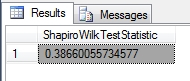
…………In Figure 3, I ran the procedure against a view created on the first 50 non-null values of the Pyruvate Kinase enzyme, derived from the 209-row table of Duchennes muscular dystrophy data I downloaded from the Vanderbilt University’s Department of Biostatistics. Given that we can’t yet calculate this on more than 50 rows at this point, doing the traditional performance test of the procedure on the HiggsBosonTable is basically pointless. Only if the lookup table could be extended somehow with new coefficients it might pay to look at the execution plan. When run against the trivial 7-row example in the Shapiro-Wilk paper, it had a couple of Clustered Index Scans that could probably be turned into Seeks with proper indexing on both the lookup table and the table being tested. It also had a couple of expensive Sort operators and a Hash Match that might warrant further inspection if the procedure could somehow be extended to datasets big enough to affect performance.
…………Interpretation of the final test statistics is straightforward in one sense, yet tricky in another. The closer the statistic is to 1, the more closely the data approaches a normal distribution. It is common to assign confidence intervals, P-values and the like with the Shapiro-Wilk Test, but I am omitting this step out of growing concern about the applicability of hypothesis testing to our use cases. I’ve often questioned the wisdom of reducing high-precision test statistics down to simple Boolean, yes-no answers about whether a particular column is normally distributed, or a particular value is an outlier; not only is it akin to taking a float column in a table and casting it to a bit, but it prevents us from asking more sophisticated questions of our hard-won computations like, “How normally distributed is my data?”
More Misgivings About Hypothesis Testing-Style Metrics
The more I read by professional statisticians and data miners who really know what they’re talking about, the less at ease I feel. Doubts about the utility of hypothesis tests of normality are routinely expressed in the literature; for some easily accessible examples that pertain directly to today’s metric, see the StackOverflow threads “Seeing if Data is Normally Distributed in R”[10] and “Perform a Shapiro-Wilk Normality Test”.[11] Some of the books I’ve read recently in my crash course in stats have not just echoed the same sentiments, but added dozens of different potential pitfalls in interpretation.[12] Hypothesis testing encompasses a set of techniques that are routinely wielded without the precision and skill required to derive useful information from them, as many professional statisticians lament. Worse still, the inherent difficulties are greatly magnified by Big Data, which comes with a unique set of use cases. The SQL Server user community might find bona fide niches for applying hypothesis testing, but for the foreseeable future I’ll forego that step and simply use the test statistics as measures in their own right, which still gives end users the freedom to implement confidence intervals and the like if they find a need.
…………The Shapiro-Wilk Test in its current form is likewise not as likely to be as useful to us as it is to researchers in other fields, in large part because of the severe limitations on input sizes. As a rule, DBAs and data miners are going to be more interested in exploratory data mining rather than hypothesis testing, using very large datasets where the means and variances are often easily discernible and sampling is less necessary. Perhaps the Shapiro-Wilk Test could be adapted to accommodate much larger datasets, as Royston apparently attempted to do by using quintic regression coefficients to approximate that constant the Shapiro-Wilk equations depend upon.[13] In fact, given that I’m still learning about the field of statistics, it is entirely possible that a better workaround is already available. I’ve already toyed with the idea of breaking up entire datasets into random samples of no more than 50 rows, but I’m not qualified to say if averaging the test statistics together would be a logically valid measure. I suspect that the measure would be incorrectly scaled because of the higher record counts.
…………Until some kind of enhancement becomes available, it is unlikely that the Shapiro-Wilk Test will occupy a prominent place in any DBA’s fitness testing toolbox. There might be niches where small random sampling and hypothesis testing might make it a good choice, but for now it is simply too small to accommodate the sheer size of the data we’re working with. I looked into another potential workaround in the form of the Shapiro-Francia Test, but since it is calculated in a similar way and is “asymptotically equivalent”[14] to the Shapiro-Wilk (i.e., they basically converge and become equal for all intents and purposes) I chose to skip that alternative for the time being. In next week’s article we’ll instead discuss the Ryan-Joiner Test, which is often lumped in the same category with the Shapiro-Wilk. After that, we’ll survey a set of loosely related techniques that are likely to be of more use to the SQL Server community, encompassing the Kolmogorov-Smirnov, Anderson-Darling, Kuiper’s and Lilliefors Tests, as well as the Cramér–von Mises Criterion
[1] Royston, Patrick, 1991, “Approximating the Shapiro-Wilk W-Test for Non-Normality,” pp. 117-119 in Statistics and Computing, September, 1992. Vol. 2, No. 3. Available online at http://link.springer.com/article/10.1007/BF01891203#page-1
[2] p. 591, Shapiro, Samuel S. and Wilk, Martin B., 1965, “An Analysis of Variance Test for Normality (Complete Samples),” pp. 591-611 in Biometrika, December 1965. Vol. 52, Nos. 3-4.
[3] See the Wikipedia page “Shapiro-Wilk Test” at http://en.wikipedia.org/wiki/Shapiro%E2%80%93Wilk_test
[4] p. 610, Shapiro and Wilk, 1965.
[5] p. 593, Shapiro, Samuel S. and Wilk, Martin B., 1965, “An Analysis of Variance Test for Normality (Complete Samples),” pp. 591-611 in Biometrika, December 1965. Vol. 52, Nos. 3-4.
[6] Apparently there is another competing definition of the term, in which values are compared within a particular column, not against across columns. See the Wikipedia page “Covariance Matrix” at http://en.wikipedia.org/wiki/Covariance_matrix#Conflicting_nomenclatures_and_notations
[7] pp. 603-604, Shapiro, Samuel S. and Wilk, Martin B., 1965, “An Analysis of Variance Test for Normality (Complete Samples),” pp. 591-611 in Biometrika, December 1965. Vol. 52, Nos. 3-4.
[8] Another source of the Shapiro-Wilk coefficient is Zaiontz, Charles, 2014, “Shapiro-Wilk Tables,” posted at the Real Statistics Using Excel blog web address http://www.real-statistics.com/statistics-tables/shapiro-wilk-table/
[9] For this part, I also consulted the National Institute for Standards and Technology, 2014, “7.2.1.3 Anderson-Darling and Shapiro-Wilk Tests,” published in the online edition of the Engineering Statistics Handbook. Available at http://www.itl.nist.gov/div898/handbook/prc/section2/prc213.htm
[10] See especially the comment by Ian Fellows on Oct. 17, 2011:
“Normality tests don’t do what most think they do. Shapiro’s test, Anderson Darling, and others are null hypothesis tests AGAINST the assumption of normality. These should not be used to determine whether to use normal theory statistical procedures. In fact they are of virtually no value to the data analyst. Under what conditions are we interested in rejecting the null hypothesis that the data are normally distributed? I have never come across a situation where a normal test is the right thing to do. When the sample size is small, even big departures from normality are not detected, and when your sample size is large, even the smallest deviation from normality will lead to a rejected null…”
…………“…So, in both these cases (binomial and lognormal variates) the p-value is > 0.05 causing a failure to reject the null (that the data are normal). Does this mean we are to conclude that the data are normal? (hint: the answer is no). Failure to reject is not the same thing as accepting. This is hypothesis testing 101.”
…………“But what about larger sample sizes? Let’s take the case where there the distribution is very nearly normal.”
…………“Here we are using a t-distribution with 200 degrees of freedom. The qq-plot shows the distribution is closer to normal than any distribution you are likely to see in the real world, but the test rejects normality with a very high degree of confidence.”
…………“Does the significant test against normality mean that we should not use normal theory statistics in this case? (another hint: the answer is no)”
 )”
)”[11] Note these helpful comments by Paul Hiemstra on March 15, 2013:
“An additional issue with the Shapiro-Wilks test is that when you feed it more data, the chances of the null hypothesis being rejected becomes larger. So what happens is that for large amounts of data even veeeery small deviations from normality can be detected, leading to rejection of the null hypothesis even though for practical purposes the data is more than normal enough…”
…………“…In practice, if an analysis assumes normality, e.g. lm, I would not do this Shapiro-Wilks test, but do the analysis and look at diagnostic plots of the outcome of the analysis to judge whether any assumptions of the analysis where violated too much. For linear regression using lm this is done by looking at some of the diagnostic plots you get using plot (lm()). Statistics is not a series of steps that cough up a few numbers (hey p < 0.05!) but requires a lot of experience and skill in judging how to analysis your data correctly.”
[12] A case in point with an entire chapter devoted to the shortcomings of hypothesis testing methods is Kault, David, 2003, Statistics with Common Sense. Greenwood Press: Westport, Connecticut.
[13] His approximation method is also based on Weisberg, Sanford and Bingham, Christopher, 1975, “An Approximate Analysis of Variance Test for Non-Normality Suitable for Machine Calculation,” pp 133-134 in Technometrics, Vol. 17.
[14] p. 117, Royston.

![]()
