By Steve Bolton

…………Throughout most of this series of amateur self-tutorials, the main topic has been and will continue to be in using SQL Server to perform goodness-of-testing on probability distributions. Don’t let the long syllables (or the alliteration practice in the title) fool you, because the underlying concept really isn’t all that hard; all these statistical tests tells us is whether the distinct counts of our data points approximate shapes like the famous bell curve, i.e. the Gaussian or “normal” distribution. While researching the topic, I found out that the term “goodness-of-fit” is also used to describe how much confidence we can assign to a particular regression line. Recall that in regression, we’re trying to learn something about the relationships between one or more variables, whereas in the case of probability distributions, we’re normally talking about univariate cases, so we’re really trying to learn something about the internal structure of a single variable (or in our case, a database column). Once again, don’t be intimidated by the big words though, because regression is really a very simple idea that every college freshman has been exposed to at some point.
…………As I explain in more detail in a post from an earlier mistutorial series, A Rickety Stairway to SQL Server Data Mining, Algorithm 2: Linear Regression, regression in its simplest form is just the graph of a line that depicts how much one variable increases or decreases as another changes in value. There are certainly complex variants of regression that could blow up someone’s brain like that poor guy in the horror film Scanners, but the fundamentals are not that taxing on the mind. Thankfully, coding simple regression lines in T-SQL is that difficult either. There are some moderate performance costs, as can be expected whenever we have to traverse a whole dataset, but the actual calculations aren’t terribly difficult to follow or debug (presuming, that is, that you understand set-based languages like SQL). That is especially true for the metrics calculated upon those regression lines, which tell us how well our data mining model might approximate the true relationships between the variables.

The Foibles and Follies of Calculating R2 and RMSE

………… Once we’ve incurred the cost of a traversing a dataset, there’s really little incentive not to squeeze all the benefit out of the trip by computing all of the relevant goodness-of-fit regression stats afterwards. For that reason, plus the fact that they’re not terribly challenging to explain, I’ll dispense with them all in a single procedure, beginning with R². In my earlier article Outlier Detection with SQL Server Part 7: Cook’s Distance we already dealt with the coefficient of determination (also known as R²), which is simply the square of the correlation coefficient. This is a long name for the very simple process of quantifying the relationship between two variables, by computing the difference for each value of the first (usually labeled X) from the average of the second (usually labeled Y) and vice-versa, then multiplying them together. This gives us the covariance, which is then transformed into the correlation by comparing the result to the product of the two standard deviations. All we need to do is implement the same code from the Cook’s Distance article, beginning with the regression calculations, then add a new step: squaring the results of the correlation. That changes all negative values to positives and thus scales the result for easier interpretation. The higher the R², the more closely the two variables are related, and the closer to 0, the less linkage there is between their values.
…………One of the few pitfalls to watch out for is that the values are often below 1 but can exceed it in some circumstances. End users don’t need to know all of the implementation details and intermediate steps I just mentioned, but the must be able to read the result, which is highly intuitive and can be easily depicted in a visualization like a Reporting Services gauge; they don’t need to be burdened with the boring, technical internals of the computations any more than a commuter needs to give a dissertation on automotive engineering, but they should be able to interpret the result easily, and R² is as mercifully simple as a gas gauge. The same is true of stats like covariance and correlation that it is built on, which costs us nothing to return to the users within the same queries.

Mean Square Error (MSE) is a little more difficult to calculate, but not much harder to interpret, since all end users need to know is that zero represents “perfect accuracy” and values further from it less fitness; the only catch might be that the goodness-of-fit moves in the opposite direction as R², which might cause confusion unless a tooltip or some other handy reminder is given to end users. Root Mean Square Error (RMSE, a.k.a. Root-Mean-Square Deviation) is usually derived from it by squaring, which statisticians often do to rescale metrics so that they only have positive values. Keep in mind that SQL Server can easily calculate standard deviation through the T-SQL StDev function, which gives us a measure of how dispersed the values in a dataset are; practically all of the procedures I’ve posted in the last two tutorial series have made use of it. What RMSE does is take standard deviation to the next level, by measuring the dispersion between multiple variables instead of just one. I really can’t explain it any better than Will G. Hopkins does at his website A New View of Statistics, which I highly recommend to novices in the field of statistics like myself:

                “The RMSE is a kind of generalized standard deviation. It pops up whenever you look for differences between subgroups or for other effects or relationships between variables. It’s the spread left over when you have accounted for any such relationships in your data, or (same thing) when you have fitted a statistical model to the data. Hence its other name, residual variation. I’ll say more about residuals for models, about fitting models in general, and about fitting them to data like these much later.”
…………“Here’s an example. Suppose you have heights for a group of females and males. If you analyze the data without regard to the sex of the subjects, the measure of spread you get will be the total variation. But stats programs can take into account the sex of each subject, work out the means for the boys and the girls, then derive a single SD that will do for the boys and the girls. That single SD is the RMSE. Yes, you can also work out the SDs for the boys and girls separately, but you may need a single one to calculate effect sizes. You can’t simply average the SDs.”[ii]

…………RMSE and R² can be used for goodness-of-fit because they are intimately related to the differences between the actual and predicted values for a regression line; they essentially quantify how much of the standard deviation or variance can be ascribed to these errors, i.e. residuals.[iii] There are many complex variants of these stats, just as there are for regression models as a whole; for example, Wikipedia provides several alternate formulas for RMSE , including some for biased estimators, which is a topic we needn’t worry as much about given the whopping sizes of the datasets the SQL Server community works with.[iv] We have unique cases in which the standard methods of hypothesis testing are less applicable, which is why I’ve generally shied away from applying confidence intervals, significance levels and the like to the stats covered in my last two tutorial series. Such tests sharply reduce the information provided by our hard-won calculations, from float or decimal data types down to simple Boolean, yes-or-no answers that a particular value is an outlier, or that subsets of values do not fit a particular distribution; retaining that information allows us to gauge how much a value qualifies as an outlier or a set of them follows a distribution, or a set of columns follows a regression line.
…………For that reason, I won’t get into the a discussion of the F-Tests often performed on our last regression measure, Lack-of-Fit Sum-of-Squares, particularly in connection with Analysis of Variance (ANOVA). The core concepts with this measure are only slightly more advanced than with RMSE and R². Once again, we’re essentially slicing up the residuals of the regression line in a way that separates the portion that can be ascribed to the inaccuracy of the model, just through alternate means. It is important here to note that with all three measures, the terms “error” and “residual” are often used interchangeably, although there is a strictly definable difference between them: a residual quantifies the difference between actual and predicted values, while errors refer to actual values and “the (unobservable) true function value.”[v] Despite this subtle yet distinguishable difference, the two terms are often used inappropriately even by experts, to the point that novices like myself can’t always discern which of the two is under discussion. Further partitioning of the residuals and errors occurs in the internal calculations of Lack-of-Fit Sum-of-Squares, but I can’t comment at length on the differences between such constituent components as Residual Sum-of-Squares and Sum-of-Squares for Pure Error, except to recommend the explanation by Mukesh Mahadeo, a frequent contributor on statistical concepts at Yahoo! Answers:

                “For certain designs with replicates at the levels of the predictor variables, the residual sum of squares can be further partitioned into meaningful parts which are relevant for testing hypotheses. Specifically, the residual sums of squares can be partitioned into lack-of-fit and pure-error components. This involves determining the part of the residual sum of squares that can be predicted by including additional terms for the predictor variables in the model (for example, higher-order polynomial or interaction terms), and the part of the residual sum of squares that cannot be predicted by any additional terms (i.e., the sum of squares for pure error). A test of lack-of-fit for the model without the additional terms can then be performed, using the mean square pure error as the error term. This provides a more sensitive test of model fit, because the effects of the additional higher-order terms is removed from the error.” It is important here to note that with all three measures, the terms “error” and “residual” are often used interchangeably, although there is a strictly definable difference between them: a residual quantifies the difference between actual and predicted values, while errors refer to actual values and “the (unobservable) true function value” chosen from a random sample.”[vi]

…………The important thing is that the code for the Lack-of-Fit Sum-of-Squares formulas[vii] gets the job done. Of course it always helps if a data mining programmer can write a dissertation on the logic and math of the equations they’re working with, but ordinarily, that’s best left to mathematicians; their assignment is analogous to that of an automotive engineers, while our role is that of a garage mechanic, whose main responsibility is to make sure that the car runs, one way or another. If the owner can drive it away without the engine stalling, then mission accomplished.
…………We only need to add two elements to make the Lack-of-Fit Sum-of-Squares code below useful to end users, one of which is to simply interpret higher numbers as greater lack of fit. The second is to define what that is, since it represents the opposite of goodness-of-fit and therefore can cause the same kind of confusion in direction that’s possible when providing RMSE and R² side-by-side. The two terms are sometimes used interchangeably, but in a more specific sense they’re actually polar opposites, in which measures that rise as fit improves can be termed goodness-of-fit and those that rise as the fit of a model declines as lack-of-fit. CrossValidated forum contributor Nick Cox provided the best explanation of the difference I’ve seen yet to date:  “Another example comes from linear regression. Here two among several possible figures of merit are the coefficient of determination R²   and the root mean square error (RMSE), or (loosely) the standard deviation of residuals. R² could be described as a measure of goodness of fit in both weak and strict senses: it measures how good the fit is of the regression predictions to data for the response and the better the fit, the higher it is. The RMSE is a measure of lack of fit in so far as it increases with the badness of fit, but many would be happy with calling it a measure of goodness of fit in the weak or broad sense.”[viii] If end users need a little more detail in what the stat means, that constitutes the most succinct explanation I’ve yet seen. Ordinarily, however, they only need to that the return values for the @LackOfFitSumOfSquares variable below will rise as the accuracy of their model gets worse and vice-versa.

Figure 1: T-SQL Code for the Regression Goodness-of-Fit Tests
CREATE PROCEDURE [Calculations].[GoodnessOfFitRegressionTestSP]
@DatabaseName as nvarchar(128) = NULL, @SchemaName as nvarchar(128), @TableName as nvarchar(128),@ColumnName1 AS nvarchar(128),@ColumnName2 AS nvarchar(128),  @DecimalPrecision AS nvarchar(50)
AS

DECLARE @SchemaAndTableName nvarchar(400),@SQLString nvarchar(max)
SET @SchemaAndTableName = @DatabaseName + ‘.’ + @SchemaName + ‘.’ + @TableName
SET @SQLString = ‘DECLARE @MeanX decimal(‘ + @DecimalPrecision + ‘),@MeanY decimal(‘ + @DecimalPrecision + ‘), @StDevX decimal(‘ + @DecimalPrecision + ‘),

@StDevY decimal(‘ + @DecimalPrecision + ‘), @Count  decimal(‘ + @DecimalPrecision + ‘), @Correlation   decimal(‘ + @DecimalPrecision + ‘),
@Covariance decimal(‘ + @DecimalPrecision + ‘), @Slope decimal(‘ + @DecimalPrecision + ‘), @Intercept decimal(‘ + @DecimalPrecision + ‘),
@MeanSquaredError decimal(‘ + @DecimalPrecision + ‘), @LackOfFitSumOfSquares decimal(‘ + @DecimalPrecision + ‘)

— STEP #1 – RETRIEVE THE GLOBAL AGGREGATES NEEDED FOR OTHER CALCULATIONS
SELECT @Count=Count(CAST(‘ + @ColumnName1 + ‘ AS Decimal(‘ + @DecimalPrecision + ‘))), @MeanX = Avg(CAST(‘ + @ColumnName1 + ‘ AS Decimal(‘ + @DecimalPrecision + ‘))),

@MeanY = Avg(CAST(‘ + @ColumnName2 + ‘ AS Decimal(‘ + @DecimalPrecision + ‘))),
@StDevX = StDev(CAST(‘ + @ColumnName1 + ‘ AS Decimal(‘ + @DecimalPrecision + ‘))), @StDevY = StDev(CAST(‘ + @ColumnName2 + ‘ AS Decimal(‘ + @DecimalPrecision + ‘)))
FROM ‘ + @SchemaAndTableName + ‘
WHERE ‘ + @ColumnName1 + ‘ IS NOT NULL AND ‘ + @ColumnName2 + ‘ IS NOT NULL

— STEP #2 – CALCULATE THE CORRELATION (BY FIRST GETTING THE COVARIANCE)
SELECT @Covariance = SUM((‘ + @ColumnName1 + ‘ – @MeanX) * (‘ + @ColumnName2 + ‘ – @MeanY)) / (@Count – 1
FROM ‘ + @SchemaAndTableName + ‘
WHERE ‘ + @ColumnName1 + ‘ IS NOT NULL AND ‘ + @ColumnName2 + ‘ IS NOT NULL

— once wee got the covariance, its trivial to calculate the correlation
SELECT @Correlation = @Covariance / (@StDevX * @StDevY) 

— STEP #3 – CALCULATE THE SLOPE AND INTERCEPT
SELECT @Slope = @Correlation * (@StDevY / @StDevX)
SELECT @Intercept = @MeanY – (@Slope * @MeanX)

— STEP #4 – CALCULATE THE MEAN SQUARED ERROR AND LACK OF FIT SUM OF SQUARES TOGETHER
SELECT @MeanSquaredError = SUM(Power((PredictedValue – ‘ + @ColumnName2 + ‘), 2)) * (1 / @Count), @LackOfFitSumOfSquares = SUM(LackofFitInput)
FROM (SELECT ‘ + @ColumnName1 + ‘, ‘ + @ColumnName2 + ‘, PredictedValue, Count(CAST(‘ + @ColumnName2 + ‘ AS Decimal(‘ + @DecimalPrecision + ‘))) OVER (PARTITION BY ‘ +
@ColumnName1 + ‘ ORDER BY ‘ + @ColumnName1 + ‘) * (Power(Avg(CAST(‘ + @ColumnName2 + ‘ AS Decimal(‘ + @DecimalPrecision + ‘))) OVER (PARTITION BY ‘ +
@ColumnName1 + ‘ ORDER BY ‘ + @ColumnName1 + ‘) – PredictedValue, 2)) AS LackofFitInput
       FROM (SELECT ‘ + @ColumnName1 + ‘, ‘ + @ColumnName2 + ‘, (‘ + @ColumnName1 + ‘ * @Slope) + @Intercept AS PredictedValue
                     FROM ‘ + @SchemaAndTableName + ‘
                     WHERE ‘ + @ColumnName1 + ‘ IS NOT NULL AND ‘ + @ColumnName2 + ‘ IS NOT NULL) AS T1) AS T2

SELECT @MeanSquaredError AS MeanSquaredError, Power(@MeanSquaredError, 0.5) AS RMSE, @LackOfFitSumOfSquares AS LackOfFitSumOfSquares,

Power(@Correlation, 2) * 100 AS R2, @Covariance AS Covariance, @Correlation AS Correlation, @Slope AS Slope, @Intercept AS Intercept‘

–SELECT @SQLString — uncomment this to debug dynamic SQL errors
EXEC (@SQLString)

…………Most of the code for this procedure is identical to that of the aforementioned Cook’s Distance procedure, which requires regression, covariance and correlation computations.[ix] I won’t rehash here how to derive the slope, intercept and other such constituent calculations, for the sake of brevity. The really striking thing is how few lines of code it takes to derive all of these incredibly useful stats in one fell swoop, which we can thank the powerful T-SQL windowing functions introduced in SQL Server 2012 for. It is noteworthy though that the outer query in Step 4 is necessary because of T-SQL error 4109, “Windowed functions cannot be used in the context of another windowed function or aggregate,” which prevents us from performing the calculations in one big gulp and plug them into the SUM. Besides a few departures like that, the procedure closely follows the format used in the last two tutorial series, in which I start with a common set of parameters that allow users to perform the test on any table in any database they have sufficient access to. The first two lines of code in the procedure body help make this happen, while the rest is dynamic SQL that begins with declarations of the constants, stats and variables we need to make the procedure perform its calculations. As usual, the @DecimalPrecision parameter is provided to help users set their own precision and scale (to avoid errors like arithmetic overflows and still accommodate columns of all sizes) and the SELECT @SQLString near the end, which can be uncommented for debugging purposes.

Figure 2: Sample Results from the Regression Goodness-of-Fit Test on the Duchennes Dataset (click to enlarge)
EXEC   [Calculations].[GoodnessOfFitRegressionTestSP]
              @DatabaseName = N’DataMiningProjects‘,
              @SchemaName = N’Health‘,
              @TableName = N’DuchennesTable‘,
              @ColumnName1 = N’Hemopexin‘,
              @ColumnName2 = N’LactateDehydrogenase‘,
              @DecimalPrecision = N’38,21′

Figure 3: Sample Results from the Regression Goodness-of-Fit Test on the Higgs Boson Dataset (click to enlarge)

EXEC   [Calculations].[GoodnessOfFitRegressionTestSP]
              @DatabaseName = N’DataMiningProjects‘,
              @SchemaName = N’Physics‘,
              @TableName = N’HiggsBosonTable‘,
              @ColumnName1 = N’Column1′,
              @ColumnName2 = N’Column2′,
              @DecimalPrecision = N’38,29′

…………I’ve made it standard practice in the last two tutorial series to test my procedures first on the 209 rows of a dataset on the Duchennes form of muscular dystrophy provided by Vanderbilt University’s Department of Biostatistics, then on the first couple of float columns in the 11-million-row Higgs Boson Dataset, which is made publicly available by the University of California at Irvine’s Machine Learning Repository. As depicted in Figure 2, the regression line for the Hemopexin protein and Lactate Dehydrogenase enzyme data in the Duchennes table fits poorly, as indicated by the MeanSquaredError, RMSE, LackOfFitSumOfSquares and R² results. The graphic below it demonstrates clearly that the first two float columns in the Higgs Boson dataset don’t fit well on a regression line either. Neither is not surprising, given that the correlation coefficients for both are near zero, which indicates a lack of relationship between the variables (a strongly negative value would indicate a strongly inverse relationship, whereas positive values would do the opposite).
…………What was truly surprising is how well the latter query performed on the Higgs Boson table, which takes up nearly 6 gigabytes in the DataMiningProjects database I assembled from various practice datasets. It only took 2:04 to execute on my clunker of a development machine, which hardly qualifies as a real database server. The execution plan in Figure 4 may provide clues as to why: most of the costs come in terms of three non-clustered index seeks, which is normally what we want to see. Nor are there any expensive Sort operators. Most of the others are parallelism and Compute Scalar operators that come at next to no cost. In last week’s article, I mentioned that it really doesn’t hurt to calculate both the Jarque-Bera and D’Agostino-Pearson Omnibus Test together, since the costs are incurred almost exclusively in traversing a whole table to derive the constituent skewness and kurtosis values. In the same way, it doesn’t cost us much to calculate the MSE, RMSE and Lack-of-Fit Sum-of-Squares together in Step 4, once we’ve already gone to the trouble of traversing the whole table by calculating one of them. It also costs us just a single operation to derive the R² once we’ve done the regression and have the correlation, and nothing at all to return the covariance, correlation, slope and intercept if we’re going to go to the trouble of getting the R². The execution plan essentially bears this out, since the Index Seeks perform almost all the work.

Figure 4: Execution Plan for the Regression Goodness-of-Fit Test on the Higgs Boson Dataset (click to enlarge)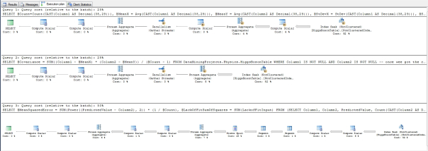

…………There are of course limitations and drawbacks with this procedure and the formulas it is meant to reflect. It is always possible that I’m not implementing them accurately, since I’m writing this in order to learn the topic, not because I know it already; as usual, my sample code is more of a suggested means of implementation, not a well-tested workhorse ready to go into a production environment tomorrow. I still lack the level of understanding I wish I had of the internal mechanics of the equations; in fact, I’m still having trouble wrapping my head around such concepts as the difference between the coefficient of determination and variance explained, which seem to overlap quite closely.[x] Moreover, the MSE can place too much weight on outliers for some use cases, even when implemented accurately.[xi] The RMSE also can’t be used to compare regressions between different sets of columns, “as it is scale-dependent.”[xii]
…………The values for the some of the stats returned above also suffer from a different scaling issue, in that they tend to increase too quickly as the number of records accumulates. They’re not in the same league as the truly astronomical values I’ve seen with other stats I’ve surveyed in the last two tutorial series, but the fact that the Lack-of-Fit Sum-of-Squares reaches eight digits above the decimal place is bothersome. That’s about the upper limit of what end users can read before they have to start counting the decimal places by hand, which rapidly degrades the legibility of the statistic.

Traditional Metrics and Tests in the “Big Data” Era

…………That just adds to my growing conviction that the vastly larger datasets in use today may require new statistical measures or rescaling of tried-and-true ones in order to accommodate their sheer size. We shouldn’t have to sacrifice the main strength of Big Data[xiii], which is the fact that we can now quickly derive very detailed descriptions of very large datasets, just to use these methods. As we have seen throughout the last two tutorial series, this issue has consistently thrown a monkey wrench into many of the established statistical procedures, which were designed decades or even centuries ago with datasets of a few dozen records in mind, not several million. We’ve seen it in the exponent and factorial operations required to derive many of well-established measures, which simply can’t be performed at all on values of more than a few hundred without leading to disastrous arithmetic overflows and loss of precision. We’ve seen it again this week and the last, in which the high record counts made the final statistics a little less legible.
…………We’ve also seen it in some of the hypothesis testing methods, which require lookup tables that often only go up to record counts of a few hundred at best. That’s a problem that will rear its head again in a few weeks when I try, and fail, to implement the popular Shapiro-Wilk Test of normality, which supposedly has excellent statistical power yet is only usable up to about 50 records.[xiv] Such goodness-of-fit tests for probability distributions can also be applied to regression, to determine if the residuals are distributed in a bell curve; cases in point include the histograms discussed in Outlier Detection with SQL Server, Part 6.1: Visual Outlier Detsection with Reporting Services and the Chi-Squared Test, which I’ll cover in a few weeks.[xv] Rather than applying these tests to regression in this segment of the series, I’ll introduce the ones I haven’t covered yet separately. For the sake of simplicity, I won’t delve into complicated topics like lack-of-fit testing on variants like multiple regression at this point. It would be useful, however, to finish off this segment of the series next week by introducing the Hosmer–Lemeshow Test, which can be applied to Logistic Regression, which is one of the most popular alternative regression algorithms. As discussed in A Rickety Stairway to SQL Server Data Mining, Algorithm 4: Logistic Regression, a logistic function is applied to produce an S-shaped curve that bounds outcomes between 0 and 1, which fits many user scenarios. Thankfully, the code will be much simpler to implement now that we’ve got this week’s T-SQL and concepts out of the way, so it should make for an easier read.

See the Wikipedia page “Mean Squared Error” at http://en.wikipedia.org/wiki/Mean_squared_error

[ii] Hopkins, Will G., 2001, “Root Mean-Square Error (RMSE),” published at the A New View of Statistics web address http://www.sportsci.org/resource/stats/rmse.html

[iii] For a more in depth explanation of the interrelationships between these stats and why they operate as they do, see Hopkins, Will G., 2001, “Models: Important Details,” published at the A New View of Statistics web address http://www.sportsci.org/resource/stats/modelsdetail.html#residuals

[iv] See the Wikipedia page “Root Mean Square Deviation” at http://en.wikipedia.org/wiki/Root-mean-square_deviation

[v] See the succinct explanation at the Wikipedia page “Errors and Residuals in Statistics” at http://en.wikipedia.org/wiki/Errors_and_residuals_in_statistics

[vi] Mukesh Mahadeo’s reply to the thread  “What is Mean by Lack of Fit in Least Square Method?” at the Yahoo! Answers web address https://in.answers.yahoo.com/question/index?qid=20100401082012AAf0yXg

[vii] Which I derived from the formulas at the Wikipedia webpage “Lack-of-Fit Sum of Squares” at http://en.wikipedia.org/wiki/Lack-of-fit_sum_of_squares

[viii] See Cox, Nick, 2013, reply to the CrossValidated thread “Are Goodness of Fit and Lack of Fit the Same?” on Aug. 2, 2013. Available at the web address http://stats.stackexchange.com/questions/66311/are-goodness-of-fit-and-lack-of-fit-the-same

[ix] As mentioned in that article, the originals sources for the internal calculations included Hopkins, Will G., 2001, “Correlation Coefficient,” published at the A New View of Statistics web address http://www.sportsci.org/resource/stats/correl.html; the Dummies.Com webpage “How to Calculate a Regression Line” at http://www.dummies.com/how-to/content/how-to-calculate-a-regression-line.html, the Wikipedia page “Mean Squared Error” at http://en.wikipedia.org/wiki/Mean_squared_error and the Wikipedia page “Lack-of-Fit Sum of Squares” at http://en.wikipedia.org/wiki/Lack-of-fit_sum_of_squares.

[x] I’ve seen competing equations in the literature, one based on residual sum-of-squares calculations and the other on squaring of the correlation coefficient. The wording often leads be to believe that they arrive at the same results through different methods, but I’m not yet certain of this.

[xi] See the Wikipedia page “Mean Squared Error” at http://en.wikipedia.org/wiki/Mean_squared_error

[xii] http://en.wikipedia.org/wiki/Root-mean-square_deviation “Root-Mean-Square Deviation”

[xiii] It’s a buzzword, I know, but it’s the most succinct term I can use here.

[xiv] Some sources say up to a couple hundred records, and I’m not familiar enough with the topic to discern which limit applies in which cases. It’s a moot point, however, because we need such tests to work on datasets of several hundred million rows.

[xv] See the undated publication “Goodness of Fit in Linear Regression” retrieved from Lawrence Joseph’s course notes on Bayesian Statistics on Oct. 30, 2014, which are published at the website of the McGill University Faculty of Medicine. Available at the web address http://www.medicine.mcgill.ca/epidemiology/joseph/courses/EPIB-621/fit.pdf. No author is listed but I presume that Prof. Joseph wrote it. This is such a good source of information for the topic of this article that I couldn’t neglect to work in a mention of it.