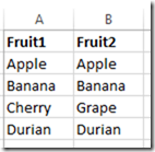
If you have two columns in an Excel sheet, and you want to conditionally format fields in the second column when the values are not equal, do this:

Our starting point – we want Grape to be highlighted because it is not the same as Cherry.
Select all of column B by clicking the header.  On the Home tab, click Conditional Formatting… New Rule.
Choose “Format only cells that contain”, and “Cell Value” “not equal to” “=A1”.  Note that putting the “=” is very important because otherwise Excel will think you’re comparing it to the string literal “A1”.

Then click “Format…” and select the appropriate formatting (such as setting a fill color).
Then click OK and OK.

Note: If you don’t want the header to be highlighted, you can apply the conditional formatting to only the cells with actual data, but you will have to adjust the corresponding comparison row in the formula.  In our example, we might apply the conditional formatting to cells B$2$:B$5$ (which starts at row 2), but we’d have to set the formula to “not equal to” “=A2” (also starts at row 2).  If you want to select down to the end of the sheet, your selection formula would be something like =$B$2:$B$1048576 on the Excel 2007+ “big grid”.