

In the previous post we looked at a one way T-Test. A one way T Test helped us determine if a selected sample was indeed truly representative of the larger population. A Two way T Test goes a step further – it helps us determine if both samples came from the same population, or if their average mean equals zero.
I am using a similar example as I did in the earlier post – but with two people. There are two walkers – A and B. They want to know if having a heavy meal has any influence on walking. Below are how many steps they took the week following thanksgiving – I , by the way, did not indulge in a heavy thanksgiving meal, but she did. Our data is as below:
| Day 1 | Day 2 | Day 3 | Day 4 | Day 5 | Day 6 | Day 7 | |
| Walker A | 10001 | 10300 | 10200 | 9900 | 10005 | 9900 | 10000 |
| Walker B | 8000 | 9200 | 8200 | 8900 | 9800 | 9900 | 9700 |
For applying the two sample T-test – we need the following conditions to be met:
1 There needs to be one continues dependant variable (walking steps) and one categorical independant variable – with two levels (whether walker had a heavy meal , or not).
2 The two samples are independant – they don’t walk together or at the same place.
3 The two samples follow normal distributions – there is no real, direct way to ensure this and there are many debates on how to determine it. For simplicity’s sake, i followed the example here – I came up with p values of under 0.05 for both walker A and B, so am good with proceeding with two sample t-test.
That done, let us define the null hypothesis, also called H0. Our null hypothesis here is that both samples have no mean difference, or in other words, the meal(s) had no influence on the differences in walking steps. The alternate, or opposite of that is that walker B walked less than walker A because he/she had a meal.
There are also parameters you need to pass to the T value function in R – if the variance of the two datasets is the same, you have to say that var.equal = true. In this case variance happens to be quite different, so we can safely leave that out and go with default T value function.
Below is the calls to the function – first from T, then TSQL, then R via TSQl. For R I did not choose to connect to SQL because the dataset in this case is seriously small.
I just open R studio and run code as below:
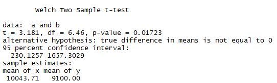
Using R:
a<-c(10001,10300,10200, 9900, 10005, 9900, 10000)
b<-c(8000, 9200,8200, 8900, 9800, 9900, 9700)
t.test(a,b)
My results are as below.
I can do the same calculation of T value using T-SQL. I cannot calculate p value from TSQL as that comes from a table, but it is possible to look it up. I imported the set of values into a table called WalkingSteps with two columns, walkerAsteps and walkerBsteps. For doing the math on T value the formula stated here may be useful. My T-SQL code is as below
Using T-SQL:
/*TSQL to calculate T value*/DECLARE @meanA FLOAT, @meanB FLOAT, @varA FLOAT, @varB FLOAT, @count int
SELECT @meanA = sum(walkerAsteps)/count(*) FROM WalkingSteps
SELECT @meanB = sum(walkerBsteps)/count(*) FROM WalkingSteps
SELECT @varA = var(walkerAsteps) FROM WalkingSteps
SELECT @varB = var(walkerBsteps) FROM WalkingSteps
SELECT @count = count(*) FROM WalkingSteps
SELECT 'T value:',((@meanA-@meanB)/sqrt((@varA/@count)+(@varB/@count)))
The result I get is as below:

To get the corresponding P value I need to stick this into a calculator, like the one here.
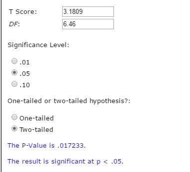
I get the same result I got with R – 0.17233. To be noted that I took the degrees of freedom from what R gave me – 6.46. If I had no access to R I’d go with 6 , as that makes logical sense. To understand more on degrees of freedom go here.
TSQL with R:
I can run the same exact R code from within TSQL and get the same results – as below:
EXEC sp_execute_external_script
 @language = N'R'
 ,@script = N'Tvalue<-t.test(InputDataSet$WalkerAsteps, InputDataSet$WalkerBsteps);
 print(Tvalue)'
 ,@input_data_1 = N'SELECT WalkerAsteps, WalkerBsteps FROM [WorldHealth].[dbo].[WalkingSteps];'
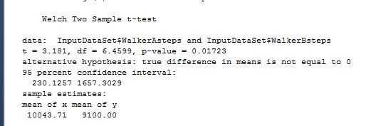
From the results we can see that the t-statistic is equal to 3.181 and the p-value is 0.007907,well below the 0.05 for the 95% confidence interval needed to accept the null hypothesis.Hence we conclude that with this data there is some evidence that a heavy meal does impact walking/exercise the week after.
I’d eat well, regardless :)) HAPPY THANKSGIVING :))

![]()
