

by Steve Bolton
The three introductory posts in this series of self-tutorials on SQL Server Data Mining (SSDM) and the separate articles on the nine algorithms Microsoft ships with it covered the most complex and essential elements of of the most under-utilized and underestimated component of the product. Most of the remaining articles in this series touch on areas that are relatively more advanced, yet which are often less complex than most of the material we’ve covered so far, and certainly less necessary to the average casual user. I’ve aimed this series mainly at the large untapped market of database professionals who aren’t statisticians by trade, but who could be using SSDM to solve real-world problems with a minimal investment of training, time, energy and server resources, including some purely relational and OLTP problems. It is more important for this class of users to expend these resources determining how to apply the right algorithms correctly in the right circumstances, not writing Data Mining Extensions (DMX) code. You can certainly make productive use of SSDM without learning any DMX, just as you can get by without becoming adept at interpreting equations. There is less incentive to dwell on the topic, but these articles on DMX will be relatively short for an equally important reason: there’s not much to say. As explained in last week’s article on performing Data Definition Language (DDL) tasks, there is far less functionality to review with DMX in comparison to T-SQL or Multidimensional Expressions (MDX), SQL Server’s relational and OLAP languages. The topic of Data Manipulation Language (DML) in DMX is a little more complex, but is still far easier to learn than T-SQL or MDX. This allows users to focus their more energy on more pressing topics, such as applying the algorithms correctly to their data.
In most SQL-based languages, the four major DML operations to take note of are UPDATE, DELETE, INSERT and SELECT statements. The same is true in DMX, but the functionality of these statements is far more limited. The meaning of the statements also differs in subtle ways. UPDATE does indeed update something, but it is merely the NODE_CAPTION of a cluster produced by the Clustering algorithm. For example, the dataset we used for example purposes throughout this series produced one named “Cluster 1” in the mining model we named ClusteringDenormalizedView1Model13, as discussed in A Rickety Stairway to SQL Server Data Mining, Algorithm 7: Clustering. To give it a new name that is more descriptive of the mining results it represents, we could use a statement like this: UPDATE ClusteringDenormalizedView1Model13.CONTENT SET NODE_CAPTION = ‘High MinuteGap Cluster’ WHERE NODE_UNIQUE_NAME = ‘001’. That’s all there is to it. We can also quickly dispose with the DELETE statement, which is designed to clear cases from either a mining model or its parent mining structure. Figure 1 succinctly explains the three different actions that can be performed using this statement. Note that the operation can be performed on either a mining structure or a model, and that the name of the specified object may be followed by a .CASES or .CONTENT keyword, which is pretty much the same pattern we’ll see with the SELECT statement. The former keyword refers to the cases used for training and the latter to those that are not.
Figure 1: Three Uses of the DELETE Statement in DMX

One use for the DELETE statement is to reclaim disk space to get rid of results from previous processing operations that are no longer needed. The most common usage scenario, however, is to empty structures or models in order to add fresh data to them using the INSERT INTO statement, which has the secondary effect of processing the objects it operates on. Contrary to the behavior of the same statement with T-SQL, you cannot use it to add new cases to a model or structure that already has any without receiving an error message; any existing data must be deleted, which severely crimps the usefulness of both DELETE and INSERT INTO. This wasteful limitation is precisely equivalent to being forced to truncate a relational table, then importing all of the same data to just to append a single new row. Likewise, inserting into a structure using syntax like INSERT INTO MyStructure is fairly straightforward because it processes the structure and all of its models, but applying it to a model in a statement like INSERT INTO MyModel is pointless if your structure has multiple models that you don’t want to process. When there is a single model in a structure, SSDM will process the model, but not its structure, unless the latter hasn’t been processed yet. Yet an error will be generated if there are any other models in the structure that need processing, so in effect, you will be forced to process any unprocessed ones anyways, which diminishes the usefulness of using INSERT INTO on a model. INSERT INTO on a structure has some performance advantages though, as former members of Microsoft’s Data Mining Team point out in their indispensable book Data Mining with Microsoft SQL Server 2008. Not only can SSDM can process all of the models efficiently by reading from the cache created in structure processing only once, but Enterprise Edition users can benefit from parallel processing of the models.
Figure 2: A Simple Example of a DMX INSERT INTO Statement
INSERT INTO MyStructure
(Column1, Column2, Column3 etc.)
OPENQUERY(DataSourceName, ‘MyQueryText’)
The second line of the INSERT INTO syntax is also upfront, in that you merely provide a comma-separated list of columns, all enclosed within parentheses, just as in T-SQL. After that, the syntax gets dicey. In the third line you must provide a comma-separated list of columns that proceeds in the same order as the corresponding columns in the first line, but this can be done through one of several different methods. One of the most common is the OPENQUERY statement, in which you provide the name of a preexisting data source and then a string used to retrieve data from it, using syntax specific to the provider the data source comes from. One of the drawbacks of this is that you can’t programmatically create the data sources, which are equivalent to the data sources we created for this tutorial series way back in A Rickety Stairway to SQL Server Data Mining, Part 0.0: An Introduction to an Introduction. The DM Team provides a complex workaround for this for adventurous users who are not faint of heart.[ii] Specifying a data source like this may not be necessary if you substitute the OPENROWSET statement, which allows you to specify the name of the provider, a connection string and the provider-specific text of your query, such as a T-SQL query. In other words, it works much like the T-SQL statement of the same name. Books Online (BOL) says you can also use other means like an MDX statement or XML for Analysis (XMLA) query, but I have yet to see practical examples of this being published anywhere, nor do I have an inkling of what syntax to use, given that I’d also have to specify the data source within them. One of the means is to use the old SHAPE statement that some of Microsoft’s data interfaces supported back at the beginning of this millennium, which is mandatory if you want to INSERT INTO nested tables. This is a complicated task which involves using five different keywords (SHAPE, APPEND, RELATE, TO and AS) in tandem with multiple parentheses and curly braces, plus your choice of access methods like OPENQUERY or OPENROWSET, which can lead to code that is both so torturous and tortuous that it makes me want to file a complaint with Human Rights Watch. All BOL says about it in each edition of the SQL Server documentation is that, “The complete syntax of the SHAPE command is documented in the Microsoft Data Access Components (MDAC) Software Development Kit (SDK).”[iii] I was tempted to say, if they’re not going to bother to document it, neither will I. The most formal yet readable example of it I have seen to date is in the DM Team book, as usual.[iv] Nevertheless I will give it the old college try and explain it as informally as possible: basically, you SHAPE { add the main query here in curly braces, such as an OPENQUERY } then APPEND ( now within parentheses, add another query here within { curly braces such as another OPENQUERY } then use a RELATE FirstQueryIDColumn TO SecondQueryIDColumn ) AS MyAlias. I’ve used it successfully before, but it’s hard to work with. If you want to use INSERT INTO with nested tables, however, learning the SHAPE command may be your only option.
Moreover, INSERT INTO has a couple of other clauses to take into account. Among these is the SKIP keyword, which can be placed next to one of the columns in the first list to indicate that the corresponding columns in your OPENQUERY or OPENROWSET query are superfluous and should be ignored, perhaps because they don’t exist in your model. This scenario pertains mainly to nested tables. The documentation also mentions a .COLUMN_VALUES clause for INSERT INTO, but it is difficult to ascertain from BOL precisely what it is used for. As I’ve mentioned before in past posts, working with SQL Server Analysis Services (SSAS) is sometimes like blasting off into space, because the documentation is sometimes so thin that you’re basically going where no man has gone before, much like Capt. James T. Kirk and Co. For example, my series of posts on An Informal Compendium of SSAS Errors is still one of the few, if not the only, centralized sources of information for certain SSAS errors, including several pertaining exclusively to data mining. The .COLUMN_VALUES is in the same category, in that I could find only four relevant hits for it in a Google search, two of which merely repeated the thin information provided in BOL. A search for it in the text of both the 2005 and 2008 editions of the DM Team’s book also turned up nada[v]. Luckily, the last hit in Google turned up a reference to a readable explanation in the original OLE DB for Data Mining Specification, written way back in July 2000, back in the days when SSDM was a brand new feature in SQL Server, with only two algorithms.[vi] Figure 3 contains a hypothetical example of the clause, which I have yet to use in practice. It supposedly allows you to supply data to one column at a time and train it aside from others, with the caveat that any related columns must be trained together. This is the closest we can get in SSDM to incremental updating, which I surmise is mostly useful for performance purposes. The OLE DB document says that “the client application can browse those values but cannot yet perform queries or browse model content,” so I don’t see what advantage having a model with incomplete results would have, except to enable this kind of crude incremental processing. BOL says that it “provides column data to the model in a concise, ordered manner that is useful when you work with datasets that contain hierarchies or ordered columns,” but I am unsure what Microsoft means by this.
Figure 3: A Hypothetical Example of the COLUMN_VALUES Clause
INSERT INTO ClusteringDenormalizedView1Model.COLUMN_VALUES
(IoStall)
OPENROWSET(‘MyProvider’, ‘MyConnectionString‘,
‘SELECT IOStall FROM MyTable‘)
Because of such complexity, you’re better off not using INSERT INTO to populate and process your models, just as you are better off creating and altering them without DMX DDL, as explained in last week’s tutorial. Typing out statements like CREATE TABLE can have some advantages in T-SQL, because it forces the query writer to think more intently about the many variables that factor into object creation and use, but this is not usually the case with DMX. The main use case for INSERT INTO, DELETE and DDL operations in DMX operations is in those situations where you’re creating and changing structures and their models on the fly, especially when the results are depicted in programs other than SQL Server Data Tools (SSDT) or earlier Visual Studio-based incarnations of it with SQL Server editions prior to 2012. A casual data miner is much more likely to depend on the GUI Microsoft provides with SSDM than they are to rely solely on SQL Server Management Studio (SSMS) to view T-SQL query results, for example. This is due in large part to the complexity of the output and the visualization tools needed to depict it, which are a lot more sophisticated than a mere spreadsheet or grid control. The next most likely usage scenario is to retrieve the raw numbers these visualizations are built with directly through a DMX query, more often in SSMS than not. Even then, however, most users will be simply selecting data from objects that have already been created and fed data in SSDT. Other use cases do occur, but they’re proportionally much less common than on the relational or even the OLAP side of things. Perhaps this is why no means was even built in to create data sources or data source views (DSVs).
Selecting data is a much more common operation in DMX, one with a bit more variety than these other DML operations but far less than corresponding SELECTs in T-SQL or MDX. The most diversity occurs in the FROM clause, which we will discuss after we get through the keywords that can be tacked on the beginning or the end of a query. This won’t take long because there are so few of them. The only keyword among them you won’t find in T-SQL is FLATTENED, which is designed mainly to denormalize DMX queries so that the NODE_DISTRIBUTION column can be depicted in GUIs that don’t supported nested tables. SSMS can depict this column correctly in DMX queries, but you can’t perform common operations like importing the data into relational tables (a crucial topic we will touch on two weeks from now) without this keyword. After this you can specify common T-SQL keywords like DISTINCT, TOP n, AS for column aliases, WHERE and ORDER BY. Their functionality is often stripped down in comparison to T-SQL, however, while in the case of DISTINCT, it is positively bizarre. When a column is specified with a Content type of Discrete (for a refresher on the crucial distinction, see the first couple of posts in this series), then it returns unique values as expected. With Continuous columns, however, it returns the median, while in the case of Discretized columns it returns the median of each bucket. The reasoning for this is quite beyond my ken. The usefulness of ORDER BY is also crimped by the fact that it can take only one condition. The operators DMX uses are mainly useful with ORDER BY and WHERE, but it features only a subset of those available with T-SQL. The language has the same arithmetic operators as T-SQL except modulo; a severely restricted subset of logical operators with AND, OR, NOT; the same comparison operators except !< and !> (not less than and not greater than); and the same unary operators, except for ~ for a bitwise NOT. Oddly, it doesn’t have this functionality, but DMX does support using // as a third means of commenting, in addition to the two used by T-SQL.
The WHERE clause can also make use of EXISTS, which is technically a function in DMX rather than a keyword. Another function which can be useful in both the SELECT list and the WHERE clause is StructureColumn(“MyColumn”), which allows you to include a column from the parent mining structure in a model that doesn’t have it, either in the SELECT results or as a filter. Lag() can also be used in a WHERE clause to retrieve “the time slice between the date of the current case and the last date in the data,” but all it does is basically take a hatchet to your dataset. Using it on any other algorithm except Time Series raises this error: “The LAG function cannot be used in the context at line n, column n.” In my limited experience, it is also allowed only in CASES queries and seems to always take the final case in the mining model as its starting point. My experience is limited precisely because I can’t find much of a practical use for it, unlike the corresponding Lag command in MDX. One of the most exciting innovations in SQL Server 2012 is the addition of analytic functions like Lag to T-SQL, which has the left the DMX version even further behind in the dust. Unlike its MDX or T-SQL counterpart, the DMX version of Lag takes no arguments, so it’s not surprising that it returns information of such little use.
Four other functions are commonly used with WHERE, including IsTestCase () and IsTrainingCase (), which take no arguments, and IsDescendant (NodeID) and IsInNode (NodeID), which you supply the parent node, or the node that you suspect contains the current case. Their functionality is fairly self-explanatory. The same is not the case with several other functions that are often used in the SELECT list, like TopCount, TopPercent and TopSum, each of which returns a table where the values for the specified column are => the count, percentile or sum. BottomCount, BottomPercent and BottomSum do the same except return the lowest values, in ascending order. They operate similar to the functions of the same name in MDX, except that the rank expression and the numerical value to check for are the second and third arguments to the function respectively, rather than the other way around. RangeMin, RangeMid and RangeMax can also be used to extract the minimum, average and maximum values for a bucket in a Discretized column. Figure 4 depicts the values returned for a Discretized column in the NBDenormalized3Model mining model used in A Rickety Stairway to SQL Server Data Mining, Algorithm 1: Not-So-Naïve Bayes. The blank first line returned with the results is a mystery to me, along with the annoying habit of SSDM to automatically insert spaces into your column names when creating mining structures, which is why we have to use brackets to enclose [Io Pending Ms Ticks] rather using the more legible name IOPendingMsTicks from my original schema. These three functions can also be used with prediction joins, in which case the results refer to the specific buckets predicted by the query.
Figure 4: Examples of RangeMin, RangeMid and RangeMax Applied to a Column in NBDenormalized3Model
SELECT DISTINCT RangeMin([Io
Pending Ms Ticks]) AS [MinIOPendingMSTicksBucket],
RangeMid([Io Pending Ms Ticks]) AS
[MidIOPendingMSTicksBucket],
RangeMax([Io
Pending Ms Ticks]) AS
[MaxIOPendingMSTicksBucket]
FROM
[NBDenormalized3Model]
Results

DMX has an entire class of prediction functions that are far more worthy of our time and attention, which deserve separate treatment next week because they are the meat and potatoes of the language. They are complemented by a specific syntax for SELECT to create what is called prediction join, which performs similar functions that it would be best to discuss separately. As depicted in Figure 5, simply selecting from a model without a CONTENT, CASES or SAMPLE_CASES clause will perform an empty prediction join, which is a topic that will also be deferred until next week. Likewise, using the DIMENSION_CONTENT clause in a FROM statement returns data from a mining dimension in a cube, which is a fairly simple topic. I will also defer that subject until after our discussion of DMX is over though, because I can augment the functionality with some custom DMX, T-SQL and MDX code that may aid DBAs who want to use SSDM successfully, without investing too much time and energy learning the whole complex metadata format I described in the posts on the individual algorithms. When you perform a CONTENT query on a model, you get back the 18 columns of that common metadata format, which vary substantially in meaning not only between algorithms but between rows, depending on the value of the NODE_TYPE column. The FLATTENED keyword is designed to denormalize the NODE_DISTRIBUTION column it returns, in which case six additional columns will be returned: ATTRIBUTE_NAME, ATTRIBUTE_VALUE, SUPPORT, PROBABILITY, VARIANCE and VALUETYPE. The meaning of these columns may also change from row to row, depending on the flag in the VALUETYPE column. For details on how to interpret these results, refer to the tutorials on each particular algorithm, which include handy charts for deciphering this rat’s nest of nested tables. Relational DBAs may be put off by this highly denormalized, flattened representation of the Generic Content Tree Viewer in SSDT, which is why I will supply code in a couple of weeks that will allow moderate users of SSDM to bypass CONTENT queries of this kind altogether. In some situations it may also be useful to inspect the cases used to train a particular structure or model, which is where the CASES clause comes into play.
One of the strangest features in DMX is the SAMPLE_CASES clause, which applies only to the Sequence Clustering algorithm. There is one sentence referring to the clause in the 2005 edition of the DM Team’s book and no mention in the 2008 edition. Beyond that, there is next to no documentation on it anywhere on the planet, except for a single cryptic note in BOL. What few sources I have found seem to agree that it returns training cases which may be generated by SSDM itself, rather than representing actual data, but I have yet to see an explanation of why Sequence Clustering would require fake cases for internal use like this. I suspect it must have something to do with constructing the Markov models it depends on, but since I lack a solid background in statistics, I can’t really say for sure. Either way, it is a bit too arcane to discuss for the purposes of this series, given that it is a poorly documented and narrowly specialized feature, which probably pertains only to rare use cases for a single algorithm that is its useful only in exceedingly specific scenarios. If you already know how to use features like SAMPLE_CASES or COLUMN_VALUES, or even need to know it, chances are you’re not in the target audience for this series of tutorials; if you’re among the select half-dozen illuminati who use it regularly, chances are you’re the guy who wrote the code. One of the puzzling things about Analysis Services is that there are so many poorly or completely undocumented features, but someone had to have written the code behind it. Sometimes, trying to backtrack and rediscover the functionality is a bit like trying to figure out where the colonists of Roanoke went from the single cryptic word they left behind, CROATOAN.
Figure 5: Types of SELECT Clauses in DMX (adapted from BOL as usual – click to enlarge)

Figure 6: The Ten Data Mining Schema Rowsets (click to enlarge)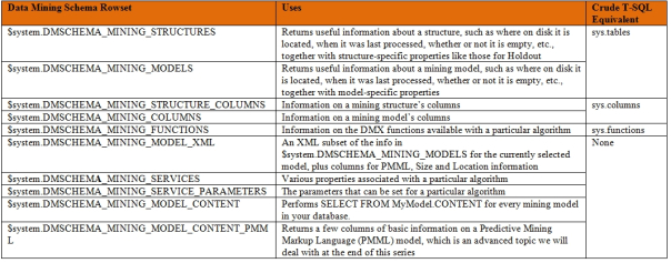
That’s almost all you need to know about DMX – with the glaring exception of prediction queries, which provide functionality that you can’t always get using the GUI in SSDT. In the remaining articles in this series we’ll also touch on some really advanced leftovers like how to call DMX stored procedures, but that can wait until we discuss their primary use case, model validation, which is one of the most important steps in a mining workflow. In the upcoming tutorial on mining dimensions, I’ll introduce an alternative that allows DBAs who are more familiar with T-SQL or MDX to slice and dice the results SSDM returns in their favorite language. There are some usage scenarios where you can’t do without DMX, but it is not an ideal tool for interpreting the results returned by the algorithms. Its functionality is simply far too limited; as I mentioned a few paragraphs up, for example, the Lag function is barbaric compared to its newborn counterpart in T-SQL. Since the multi-dimensional data SSDM deals with is so complex, you would assume that DMX wouldn’t be so simplistic and one-dimensional. Perhaps it is still in its infancy as a language, just as the whole data mining field is, or perhaps it has died stillborn for lack of attention from the top brass at Microsoft, given that it hasn’t been updated much since SQL Server 2005. I look at it as the proper tool to do one of two jobs, the first of which is to get my mining data into relational tables or cubes, where I can perform operations on it that are more useful and sophisticated by several orders of magnitude, using T-SQL and MDX. The second of these is to perform prediction queries, which is the real raison d’être of the language and gives SSDM a whole new level of functionality that isn’t necessarily possible in the GUI.
p. 109, MacLennan, Jamie; Tang, ZhaoHui and Crivat, Bogdan, 2009, Data Mining with Microsoft SQL Server 2008. Wiley Publishing: Indianapolis.
[ii] IBID., pp. 109-110.
[iii] See the MSDN webpage “SHAPE (DMX)” - http://msdn.microsoft.com/en-us/library/ms131972.aspx
[iv] pp. 110-112, MacLennan, et al.
[v] IBID. Also see MacLennan, Jamie andTang, ZhaoHuin, 2005, Data Mining with Microsoft SQL Server 2005. Wiley Publishing: Indianapolis.
[vi] pp. 37-38, Microsoft Corporation, 2000, OLE DB for Data Mining Specification Version 1.0. Available online at Dwight Calwhite’s website at www.calwhite.com/files/OLEDBDM1.doc

![]()
