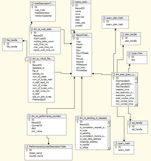
As I mentioned in A Rickety Stairway to SQL Server Data Mining, Part 0.0: An Introduction to an Introduction, I’m not going to waste much time in this series on self-explanatory steps, such as how to create a project in SSDT, since the topic is complex enough. In that introductory post I also succinctly summarized the process of creating a project, followed by a data source, a data source view, a mining structure and then mining models, in that order; please refer back to it if necessary. In many projects it may be preferable to create a cube from the data source views and then build mining structures on top of that, but I’m skipping that step to reduce the complexity of the tutorials. To make a long story short, I created a MonitorMiningProject, a data source called MonitoringDS and the data source view (DSV) depicted above. Note that most of the columns depicted in the DSV have the same names and data types as those associated with dm_exec_query_stats, dm_io_pending_io_requests, dm_io_virtual_file_stats, dm_os_performance_counters, dm_os_wait_stats and sp_spaceused in Books Online (BOL). I did make a few changes, however, in order to normalize some of the bloated tables, which enabled me to reduce the size of the database to 2.8 GB. I put the file_handle, wait_type, counter_name, sql_handle, plan_handle, text, query_hash, and query_plan_hash columns of dm_io_virtual_file_stats, dm_os_wait_stats, dm_os_performance_counters and dm_exec_query_stats in their own separate tables, then joined those to the original tables on new columns called FileHandleID, WaitStatID, CounterID, SQLHandleID, PlanHandleID, QueryTextID, QueryHashID and QueryPlanHashID. At present we only need to record the fact that a particular query plan, query text, file handle, etc. was associated with other performance data or event; preserving the binary or text data that the new foreign keys point to might come in handy after the data mining process is finished, however, if we find a plan handle or query text associated with interesting data. These subordinate tables are included in the DSV so that we can, for example, look up a particular plan handle or query text, but there’s no need to perform any direct mining on them. Other changes included stripping the varchar columns that sp_spaceused produces of the letters ” KB” and casting the columns to bigint, as well as changing the varbinary columns returned by dm_io_pending_io_requests to bigint. The first step put the numeric data in the sp_spaceused columns in a usable form that can be designated with the Continuous content type, while the latter got around a restriction SQL Server Analysis Services (SSAS) has against using varbinary columns.

          I will be using the schema depicted in Figure 2 for the rest of the tutorial series, unless the need arises to change it, as it probably will. On the Specify Training Data page of the Data Mining Wizard (which is discussed in more depth in previous posts) I left out some columns in the RecordTableView that I don’t really need, like Second, Month, Week, Year and Millisecond. For purposes of simplicity and legibility, I used a single integer identity column named ID as the clustered primary key in each table, all of which were designated in the Wizard as Key columns. In previous posts I wrote that I would save the topic of nested tables for an upcoming article on Sequence Clustering, but because all of my tables were joined to a single master table, it seemed appropriate to designate all of the child tables as nested relations of the RecordTableView. As we shall see, I should have followed my original instinct and put off using nested tables for later in this series, because they turned out to be the source of my performance problems. All of the columns of these subordinate tables were set as both Input and Predictable attributes, i.e. the data that will be input and output by SSDM; for a more in-depth discussion of them, see my previous posts in this series. The measures of time in the RecordTable were set to Input only, since we don’t need to predict anything about them. Figure 2 provides a summary of the schema we’ll be using for the rest of this series:

Figure 2: The DSV Schema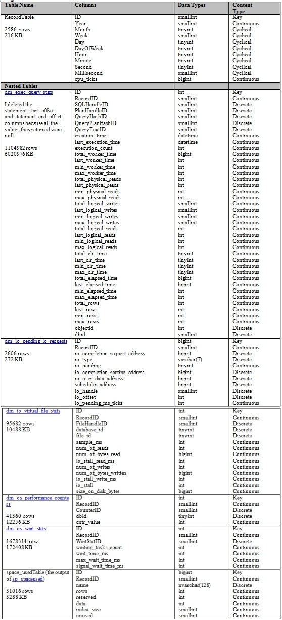

           As I mentioned in the previous two posts, the tricky part is setting the Content Type of each column correctly. That calls for thinking about the meaning of your data in subtle ways OLTP DBAs might be less familiar with. In Figure 2, the key columns are all designated with a Key type, which is a no-brainer. The rest of the designations take a little more thought though. Most of the columns in the RecordTableView are designated as Cyclical because they only accumulate to a point, then repeat themselves, as the Minute counter does each hour, for example. Year and cpu_ticks columns, for example, are cumulative integer counters that imply both a rank and an order to the numbers, therefore they are designated as Continuous. When a column represents a cumulative measure of some kind that doesn’t repeat itself the way that Cyclical measures like DayOfWeek do, that is a dead giveaway that it ought to be set to Continuous whenever possible. Most of the remaining columns in Figure 2 are set to Continuous for that reason, including RecordID, which doubles as an ordered, cumulative measure of trials – except without a definite rank, thanks to the gaps introduced when SSIS skipped data collection jobs. A handful of others are set to Discrete, such as WaitStatID; CounterID; dbid; FileHandleID; database_id; file_id; SQLHandleID; PlanHandleID; QueryHashID; QueryPlanHashID; QueryTextID; objectid; io_completion_request_address; io_type; io_completion_routine_address; io_user_data_address; scheduler_address; io_handle; io_offset. At the last minute, I had to change the Content type of the IO Pending column to Discrete rather than Discretized because of an error message that read, “attribute with ID of ‘Io Pending’, Name of ‘Io Pending’ cannot be discretized because there are too few distinct values.” Sure enough, I checked the results and it had a constant value of 1 throughout the data collection phase. Except for that aberrant IO Pending column, what they all have in common is that they represent specific objects without implying a rank or order among them. In principle, you might have reason to assign a rank or order between one plan handle and another, or one database file and another, but these columns only record the fact that they are separate entities. Unique values in a Discrete column are independent of each other, in the same way that “M” and “F” simply represent different, independent states in a Gender column. Such independence might be a problem, however, if “M” and “F” were meant to designate a Continuous relationship among the distinct values, such as alphabetical ordering. Unfortunately, some of the Microsoft algorithms, like Naïve Bayes, cannot make use of Continuous columns, so those must be treated as Discrete columns through a process known as discretization, which can be tweaked with a few mining model parameters. Some algorithms likewise do not support Cyclical, Ordered and Key Sequence types, and in these cases, we will adapt the model in Figure 2 accordingly.

Problems and Practice with Parameters and Performance

      I had to do a lot more adaptation than I expected, due to unforeseen performance issues. I was accustomed to running all nine algorithms on smaller datasets of a few thousand rows in a single table, with little performance impact on my creaky development machine, so I did not expect to encounter some of the problems that arose while processing the data, training the algorithms and then retrieving the results. Each of these steps brought either my Analysis Services instance, SQL Server Data Tools (SSDT), SQL Server Management Studio (SSMS) or my machine to their knees at various times. I did some smoothing of my data before attempting to process the mining model for the first time, such as normalizing the data returned by the dynamic management views (DMVs), but that was not sufficient to prevent msmdsrv.exe from gobbling up all 8 gigs of RAM, then 40 gigs of page files before it crashed during the processing phase. This led to Lesson #1: Watch your Disk Activity in Resource Monitor to see what files are being hit and the Active Time and Disk Queue Length counters to see if you’re getting excessive disk activity during processing or algorithm training; if so, try moving TempDB, the SSAS Temp folder and your database folder to an SSD. That dramatically improved the initial phase of processing in this trial, to the point that msmdsrv.exe still crashed, but without bringing the machine to a grinding halt with it. SSAS wouldn’t quit per se, but would instead hang for hours on end during the algorithm training phase, by maxing out one core without the memory or IO counters in Task Manager budging. The sheer volume of data I was feeding it was apparently just too much for it to handle. The situation didn’t improve any until I learned Lesson #2: Shrink the data types in your dataset to the minimum possible size, based on the actual data returned. For example, the DMVs returned some bigint and int columns that I was able to shrink to smallints and tinyints because the values returned were sufficiently small. After going through my schema with a fine-toothed comb, using a query I devised to find shrinkable columns (which I will eventually post here), I was able to drastically reduce the amount of RAM consumption, paging and IO activity by msmdsrv.exe. Model processing would now complete but I wasn’t able to get the algorithm training phase to terminate, however, until I scaled back the size of my data mining models by comparing only a couple of tables at a time. Apparently the schema in Figure 1, with its six nested tables and millions of rows, was too ambitious for a six-core desktop development machine. That led to Lesson #3: Partition your data mining trials by creating separate mining models for subsets of your columns and nested tables. For example, after I cut back to just comparing dm_io_pending_io_requests and dm_io_virtual_file_stats, I was able to complete the algorithm training phase at last.

     At this point, I expected to be able to view the results in the Naïve Bayes Content Viewer and Generic Content Viewer, but then another unexpected problem reared its head: neither SSMS nor SSDT could handle the volume of results without crashing. Throughout this phase of troubleshooting the window depicted below would appear in either one of these tools and then spin for hours. Initially it wouldn’t even do this until I removed the connection timeouts in the SSMS Connect to Server and in the Tools/Options menu item in SSDT, where it can be found under the Business Intelligence Designers/Analysis Services Designers/General node when Show all settings is checked. After that, the dial in the window below would spin for hours while msmdrv kept plugging away, until SSDM or SSDT simply restarted on their own without warning.

Figure 3: The Sending Query to Server Window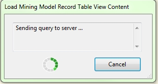

                After this I went on another hunt for redundant information to slim down the model some more. I noticed that only two values were present in io_type, “disk” and “network,” but knew from experience that the latter was just part of normal background processing and was therefore of no consequence. That led to Lesson #4: Use the mining model’s Filter property to eliminate unnecessary data before processing. This allows you to set a WHERE filter that isn’t as useful as the corresponding T-SQL clause, but can still get the job done. I was then able to discard io_type because there was only one value left, as well as io_completion_routine_address, which only varied with the network io_type. I also spotted two mistakes I should have caught earlier: io_pending only had one value as well, plus sample_ms was basically redundant because the system time was already recorded in the RecordTable each time the SSIS job ran. After applying Lesson # 5: Continually check for unimportant or redundant data that can be discarded, I was at last able to get to the point where SSMS and SSDT sometimes at least returned error messages instead of restarting without warning. In SSDT, this sometimes took the form of the message “An error occurred while the mining model was being loaded. Internal .Net Framework Data Provider error 12.” In SSMS, attempting to return the full results in an MDX query led to the message Server: The operation has been cancelled because there is not enough memory available for the application.” Sure enough, prior to each occurrence of these messages RAM consumption would rapidly rise like a rollercoaster heading for the peak of its track. Lesson #6: Keep your eye on available RAM in Task Manager already seemed self-evident to me before this experiment began, but I’ll repeat it here anyways. I expected RAM consumption to spike during the processing and algorithm training phases, but it never occurred to me that it would be a problem when retrieving the results.

          After this, the necessity of choosing the right inputs, predictables, parameters and data schema came to the fore. Since performance had already become an issue even at this early stage, using the simplest of the nine SSDM algorithms, I also decided to put off on any experimentation with the various parameters that can be used to tweak the algorithms, but the need to adjust them became evident when both crashed repeatedly due to the sheer size of the results. Scaling down the dataset allowed the processing job for the mining model to complete, but SSDT and SSMS simply couldn’t represent all of the results in their GUIs without choking. I’m assuming that this was most likely due to the high number of distinct values and wide variance and standard deviation within the columns of both dm_io_pending_io_requests and dm_io_virtual_file_stats, in which case the only alternative left seemed to lay in the parameters available for Naïve Bayes, all of which are available for the other eight algorithms. The only mining model flags available for this algorithm weren’t germane to the problem because they’re for simple null handling. None of our data should have nulls, but if some are present, it doesn’t really affect the quality of the data, so there is no point setting the NOT NULL flag. For our purposes, setting the MODEL_EXISTENCE_ONLY flag would only serve to strip our data of any meaning by treating it at as either Missing or Existing, rather than considering the actual values.

          I initially held the view that the parameters MAXIMUM_INPUT_ATTRIBUTES and MAXIMUM_OUTPUT_ATTRIBUTES weren’t relevant either, since I had fewer than 255 columns in my schema, even before scaling it back to dm_io_pending_io_requests and dm_io_virtual_file_stats. I therefore left them at their defaults values of 255, which I believed would prevent SSAS from using a means of complexity reduction known as feature selection to improve performance. This involves a tradeoff between the quality of results and performance and is achieved by using one of four methods: the interestingness score, Shannon’s Entropy, Bayesian with K2 Prior and Bayesian Dirichlet Equivalent with Uniform Prior. The first of these is calculated by giving greater weight to data distributions which are non-random, but it is only available for Continuous columns, which aren’t compatible with Naïve Bayes. Shannon’s Entropy is a probability-based method that Naïve Bayes can use because it is compatible with Discrete and Discretized values; the precise formula is cited at the Books Online page Feature Selection (Data Mining).  Naïve Bayes can also make use of the latter two methods, which are themselves based on Bayesian calculations derived from the aforementioned methods devised by Heckerman, et. al. Another reason I’m going to postpone discussion of them is that at this point, I have yet to find a way to discern which of the three methods SQL Server is applying under the hood. With certain algorithms it is possible to return the interestingness score in the MS_OLAP_NODE_SCORE column in the results, but that’s the only method I’ve found yet. I’m also too unfamiliar with the inner workings of feature selection to have a good feel for the optimum settings for MAXIMUM_INPUT_ATTRIBUTES and MAXIMUM_OUTPUT_ATTRIBUTES, which led to a lot of time-consuming trial-and-error on my part. At one point it I began to believe that they affected the number of distinct states in each predictable and input column, rather than merely capping the number of columns, because I shouldn’t have had anywhere near 255 attributes; on the other hand, MAXIMUM_STATES is the parameter is supposed to limit the number of distinct states, not the two attribute parameters. The solution to this mystery became evident later, as I will soon discuss. For awhile, however, it seemed as if SSMS and SSDT were sputtering because I had still had 13 columns left in my reduced structure with more than a thousand unique values, many of which had exceptionally wide standard deviations and variances according to the output of the T-SQL functions StDev and Var. Once I limited the number of input or predictable attributes for both by reducing them from their default values to 128, I began receiving messages upon the completion of model processing that “Automatic feature selection has been applied to model, NaiveBayesModel due to the large number of attributes.” Strangely, I still received it after I switched to another mining model comparing dm_io_pending_io_requests and dm_os_performance_counters and set both parameters to zero, which should have disabled feature selection.

          Another warning may also appear several times in between the completion of algorithm training and the retrieval of results, stating that  “Cardinality reduction has been applied on column” such-and-such “of model, NaiveBayesModel due to the large number of states in that column.  Set MAXIMUM_STATES to increase the number of states considered by the algorithm.” This should only be present if the MAXIMUM_STATES parameter is not set to zero, which will cap the total number of states that a column can have before SSAS discards the less numerous ones and designates them as Missing, with the default value being 100.  MINIMUM_DEPENDENCY_PROBABILITY can also be used to reduce the number of attributes for a model by requiring higher probability thresholds to keep a state from being discarded. Lower values on a scale from 0 to 1 lead to more attributes and consequently, higher risk of performance issues or information glut, with the default being 0.5. The DiscretizationBucketCount and DiscretizationMethod properties also provide alternatives means of optimization, at least with Discretized columns. The first determines the number of buckets that discretized columns will be grouped into; for example, if you have a column with values ranging from 1 through 5 and DiscretizationBucketCount is set to its default value of 5, we can evenly distribute the five values into separate buckets. When using a cube, SSAS automatically assigns the number of buckets based on the square root of the distinct values in that column. The DiscretizationMethod determines how the values are divided. EQUAL_AREAS splits the data into groups of equal size, which doesn’t work well on lopsided data. In that case we might want to use CLUSTERS, which is better suited for such cases. As BOL says, it involves taking a random sample of 1,000 records and “then running several iterations of the Microsoft Clustering algorithm using the Expectation Maximization (EM) clustering method,” but this is more resource-intensive. For now I will leave it set to AUTOMATIC, which allows SSAS to choose the best method. In most scenarios I’ve seen at Microsoft’s Data Mining Forum, the HoldoutSeed is left at either 20 or 30 percent of the data, so for now I’ll leave it at the latter value. We may revisit all of these parameters in the future to see how a little tweaking can affect the performance and quality of results, but my main concern at this point was just to whittle the dataset down enough to get SSDT or SSMS to return any results at all without crashing. In past projects I’ve used much smaller datasets where this wasn’t an issue, but my methodology in this series was to test SSDM’s limits on a small machine and I simply got more than I bargained for. If all goes as planned, throughout this series I will gain a better sense of how to set all of these properties to maximize performance and the usefulness of the results, but at present I’m stuck with a lot of trial-and-error, which means a long trial and plenty of errors.

          The curious thing was that every trial seemed to end in errors, no matter how I set the above parameters. Even when I set the two attribute parameters to ridiculously low values like 16, while simultaneously taking MAXIMUM_STATES down to 5 and MINIMUM_DEPENDENCY_PROBABILITY up to 0.75, performance was still quite poor. If results came back at all, they were meaningless. Eventually it dawned on me that the nested tables were causing an exponential explosion in the number of attributes the model was processing, thereby leading to performance problems and meaningless results. As noted before, my experience with nested tables was limited to the Sequence Clustering algorithm, so I was unprepared for this particular problem; I expected, however, that they would improve performance for the same reasons that normalization does. Yet even my MDX queries were crashing unless I used really restrictive WHERE clauses, so I had trouble even looking under the hood to see what the culprit was. In one of these queries, I was astounded to see that SSDM had generated several hundred thousand attributes for a simple comparison of dm_io_pending_io_requests and dm_os_performance_counters, both joined to the RecordTable, totaling just 320 rows. At this point, I could view the Generic Content Viewer in SSDT as long as I didn’t click on certain parent nodes, but two of the other tabs were simply blank because it simply couldn’t handle the sheer number of results. One of the key principles of troubleshooting is to check for any variables you’ve recently changed since things went awry, so it seemed likely that the nested tables were to blame. So I created a denormalized view of those two tables joined to their mutual parent, then threw in dm_io_virtual_file_stats for good measure. The single view that replaced these three nested tables and their parent had about 720 rows in common through INNER JOINs, or more than double what I had in the last pared-down trial. Yet it finished almost instantly, without feature selection being invoked or cardinality warnings arising, even with all of the parameters set back at their default values. I have yet to learn enough about nested tables in SSDM to explain why this exponential growth in attributes occurred, but we will revisit the issue before the end of the series, perhaps in a separate post around the time I post on the Sequence Clustering algorithm. This led to Lesson #7: Experiment with denormalizing your nested tables if the number of attributes goes through the roof.

          As I will share in the future, I have gotten some quite useful results while operating on data of tables of a few hundred or few thousand rows, but this was the first time I had run a data mining trial on two gigs of data spread out over several nested tables, some of which had more than a million rows and a long list of columns. I assumed the performance problems came from the sheer size of the data, when the culprit was actually the fantastic growth in the number of attributes from using nested tables. This is a bit counter-intuitive, given that normalization usually leads to better performance in the OLTP world, but in this case neither processing nor useful results were possible without denormalization. Although you would normally reuse the same relationships found on the relational side when creating a DSV, SSDM apparently treated nested tables differently than a relational system does:

          “In the case table, the key is often a customer ID, a product name, or date in a series: data that uniquely identifies a row in the table. . However, in nested tables, the key is typically not the relational key (or foreign key) but rather the column that represents the attribute that you are modeling.”

          “For example, if the case table contains orders, and the nested table contains items in the order, you would be interested in modeling the relationship between items stored in the nested table across multiple orders, which are stored in the case table. Therefore, although the Items nested table is joined to the Orders case table by the relational key OrderID, you should not use OrderID as the nested table key. Instead, you would select the Items column as the nested table key, because that column contains the data that you want to model. In most cases, you can safely ignore OrderID in the mining model, because the relationship between the case table and the nested table has already been established by the data source view definition.”

          “When you choose a column to use as the nested table key, you must ensure that the values in that column are unique for each case. For example, if the case table represents customers and the nested table represents items purchased by the customer, you must ensure that no item is listed more than one time per customer. If a customer has purchased the same item more than one time, you might want to create a different view that has a column that aggregates the count of purchases for each unique product.”

           “How you decide to handle duplicate values in a nested table depends on the mining model that you are creating and the business problem that you are solving. In some scenarios you might not care how many times a customer has purchased a particular product, but want to check for the existence of at least one purchase. In other scenarios, the quantity and sequence of purchases might be very important.”[1]

                My one claim to fame as a novice is that at one point or another, I had all the Books Online documentation for the last few versions of SQL Server memorized, but somewhere along the line missed this important point. I will have to research the precise way in which SQL Server calculates the number of attributes, columns and states to be able to produce benchmarks and accurately forecast bottlenecks. That task can be put off until we discuss Sequence Clustering much later in this series. Now that I’ve managed to dig out of the data mining cave-in and avoided an epic fail, we can proceeded with our regular scheduled program: A Rickety Stairway to SQL Server Data Mining, Algorithm 1: Not-So-Naïve Bayes. A couple of days after that (barring attacks by rogue dust bunnies and mutant bacteria) it will be time to take the next step up the stairway, to a data mining method of a little more complexity, in A Rickety Stairway to SQL Server Data Mining, Algorithm 2: Linear Regression.