Introduction

I'm currently working on a 1.2T data warehouse (DWH) where the main transaction table has reached 1.5 billion rows (around 400G in size) and is growing by approximately 2 million rows a day. This table is partitioned and the data is stored as page compressed. The hardware has been correctly sized. Just to mention what is it:

• 198G RAM
• 24 cores
• 48 x 10K rmp 300G HDs configured in multiple (12) RAID10s for the data files.

Performance for the whole DWH is OK, however, lately we started to experience some problems.

1. Statistics re-computations on the transaction table are taking a long time.
2. DBCC CHECKDB or DBCC CHECKTABLE are also taking too long. Yes, I'm using the EXTENDED_LOGICAL_CHECKS and DATA_PURITY options to perform more thorough checks and I'm aware that when using these options, more time is needed to execute the checks. However, my priority is to make sure that the DB is not corrupted. To get the checking done, I'm having to split the DB checking across multiple days, specifically during the weekend when the users accessing the system are the lowest.
3. Wrong, or less efficient, plans are being selected by the optimizer. I have noticed that this is happening because the statistics (even after a FULL SCAN) are presenting a distorted data distribution picture to the optimizer. Remember that the statistics histogram is only 200 steps, regardless of the number of rows in the table.

The DWH is still in its early stages of development, and it's being accessed by SSRS reports as well as being processed by an OLAP cube. No other applications exist which query/access the DWH. I had been aware that this fact table will grow significantly and quickly, and therefore I had already preempted that I may need to use partitioned views besides table/index partitioning to help me manage better this table. In fact, all querying on this fact is already done through a view, which is one of the many pre-requestions for using partitioned views. You can find all the table/columns rules for partitioned views here.

Before delving into development and making any changes, I needed to make a proof of concept about partitioned views. I needed to prove that partitioned views will improve managibility on this huge table especially the related maintenance tasks.

As with all development changes and improvements, a balance must be found between the amount of development effort and the time needed to perform these changes. In this case I struck a balance and will be benefiting from the multiple data split across table members, but without making any PK, FK changes. Meaning that I would not be able to update directly the view. In my case, this will not be an issue because the 'last' updatable table will always be called the same and therefore will break no processes, specifically the SSIS ETL packages.

This article is a description of the changes I made to test things out together with my observations.

Real life example

As mentioned in the introduction, I'll be basing my test on the Transaction table, however with a smaller subset of data. Since I'll be doing these tests on my development environment, this not being as powerful as my production, I could not load 1.5 billion rows into the dev database. Instead, I loaded a modest 141 million rows.

In this table I have 5 years of data with the data almost balanced across the years. I will split the table by year, i.e. I'll create 5 tables and distribute the data across. 

CREATE TABLE [dbo].[FactTransaction](
[TransactionSK] [bigint] IDENTITY(10,1) NOT NULL,
.
.
[CustomerFK] [int] NOT NULL,
[TransactionDateFK] [int] NOT NULL
 .
 .
CONSTRAINT [PK_FactTransaction] PRIMARY KEY CLUSTERED 
([TransactionSK] ASC)
WITH (PAD_INDEX = OFF, STATISTICS_NORECOMPUTE = OFF, IGNORE_DUP_KEY = OFF, ALLOW_ROW_LOCKS = ON, ALLOW_PAGE_LOCKS = ON) ON [PRIMARY]
) ON [PRIMARY]

The table below details the new tables, showing the data distribution and check constraint which I created on the TransactionDateFK (YYYYMMDD) columns.

Notes:

• An Index has been created on all tables, on the CustomerFK column.
• FactTransaction_ALL is the original table containing all records. I've used this table to compare my tests against.
• FactTransaction is the current year table, i.e. 2013 in this case.

A new view v_FactTransactionBase will be used to UNION ALL base tables (obviously except the FactTransaction_ALL). 

SELECT *
    FROM dbo.FactTransaction_2009
UNION ALL
SELECT *
    FROM dbo.FactTransaction_2010
UNION ALL
SELECT *
    FROM dbo.FactTransaction_2011
UNION ALL
SELECT *
    FROM dbo.FactTransaction_2012
UNION ALL
SELECT *
    FROM dbo.FactTransaction

OK, so let's check what's actually happening...

Throughout all scenarios, I'm displaying the IO Statistics to get an overview of the logical reads and also enabled the Actual execution plan.

1) Scenario 1

For this scenario, I have selected 10 customer FKs who have transactions (intentionally) only in the last table, i.e. FactTransaction. Note that I have specified a date condition (which is similar to the column constraints).

SET STATISTICS IO ON
SELECT CustomerFk
    FROM FactTransaction_ALL
    WHERE CustomerFk IN ( 3175951, 1354109, 4788840, 5426872, 598353, 1300747,
                          3838935, 1300129, 1299711, 431263 )
        AND TransactionDateFK = 20130102
SELECT CustomerFk
    FROM dbo.v_FactTransactionBase
    WHERE CustomerFk IN ( 3175951, 1354109, 4788840, 5426872, 598353, 1300747,
                          3838935, 1300129, 1299711, 431263 )
        AND TransactionDateFK = 20130102
SET STATISTICS IO OFF

Looking at the STATISTICS IO below, it is evident that the first SELECT needed to read more data pages (126,128) to return the result set. On the other hand, the 2nd SELECT statement returned exactly the same result set but automatically did all the reading using the last table, i.e. FactTransaction (which contains 2013 data only) and needed 22,779 pages to satisfy the query. This is a huge difference which is translated to a performance increase.

(75 row(s) affected)

Table 'FactTransaction_ALL'. Scan count 10, logical reads 126128, physical reads 0, read-ahead reads 0, lob logical reads 0, lob physical reads 0, lob read-ahead reads 0.

(1 row(s) affected)

(75 row(s) affected)

Table 'FactTransaction'. Scan count 10, logical reads 22779, physical reads 0, read-ahead reads 128, lob logical reads 0, lob physical reads 0, lob read-ahead reads 0.

(1 row(s) affected)

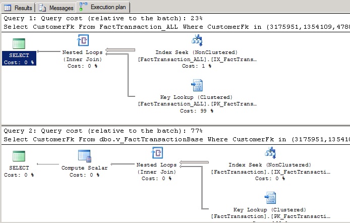
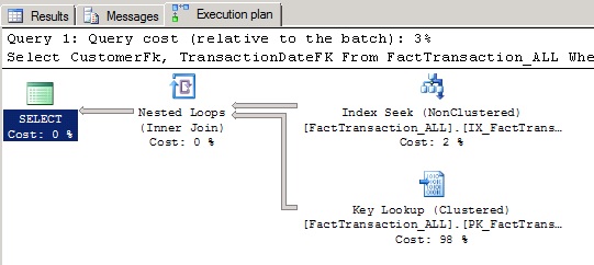
Taking a look at the below execution plan, it becomes more obvious why less data pages were read to satisfy the same query. In the first SELECT, the whole table/index was read and then a key lookup was performed to get the TransactionDateFK column.

In the 2nd SELECT, the data was also read from the index however only the affected table/index was scanned. In fact, only the last member table was scanned, this being much smaller in size. The optimizer automatically determined that it could get all the data from just one of the tables.

2) Scenario 2

For this scenario, I have selected 2 customer FKs who have transactions (intentionally) in all partiton tables, i.e. FactTransaction. Note that this time I have not specified a transaction date and therefore all the tables will need to be scanned to retrieve the data.

SET STATISTICS IO ON
SELECT CustomerFk
      , TransactionDateFK
    FROM FactTransaction_ALL
    WHERE CustomerFK IN ( 1455099, 27549 ) 
SELECT CustomerFk
      , TransactionDateFK
    FROM v_FactTransactionBase
    WHERE CustomerFK IN ( 1455099, 27549 ) 
SET STATISTICS IO OFF

(4660 row(s) affected)

Table 'FactTransaction_ALL'. Scan count 2, logical reads 18957, physical reads 0, read-ahead reads 0, lob logical reads 0, lob physical reads 0, lob read-ahead reads 0.

(1 row(s) affected)

(4660 row(s) affected)

Table 'Worktable'. Scan count 0, logical reads 0, physical reads 0, read-ahead reads 0, lob logical reads 0, lob physical reads 0, lob read-ahead reads 0.

Table 'FactTransaction'. Scan count 2, logical reads 8, physical reads 0, read-ahead reads 0, lob logical reads 0, lob physical reads 0, lob read-ahead reads 0.

Table 'FactTransaction_2012'. Scan count 2, logical reads 3328, physical reads 0, read-ahead reads 0, lob logical reads 0, lob physical reads 0, lob read-ahead reads 0.

Table 'FactTransaction_2011'. Scan count 2, logical reads 2583, physical reads 0, read-ahead reads 0, lob logical reads 0, lob physical reads 0, lob read-ahead reads 0.

Table 'FactTransaction_2010'. Scan count 2, logical reads 3194, physical reads 0, read-ahead reads 0, lob logical reads 0, lob physical reads 0, lob read-ahead reads 0.

Table 'FactTransaction_2009'. Scan count 2, logical reads 9896, physical reads 0, read-ahead reads 0, lob logical reads 0, lob physical reads 0, lob read-ahead reads 0.

(1 row(s) affected)

Looking at the above statistics, 18,957 reads were needed to retrieve and satisfy the first query (FactTransaction_ALL), while 19,009 reads were requested to satisfy the 2nd query (Partioned View). From these figures we can conclude that the 2nd query requested slightly more reads, so it is therefore slightly less efficient. However, here we're talking about 52 pages only, which are insignificant (at least in my opinion). This was predictable since now all the member tables needed to be scanned to retreive the data because the partitioning column was not specified.

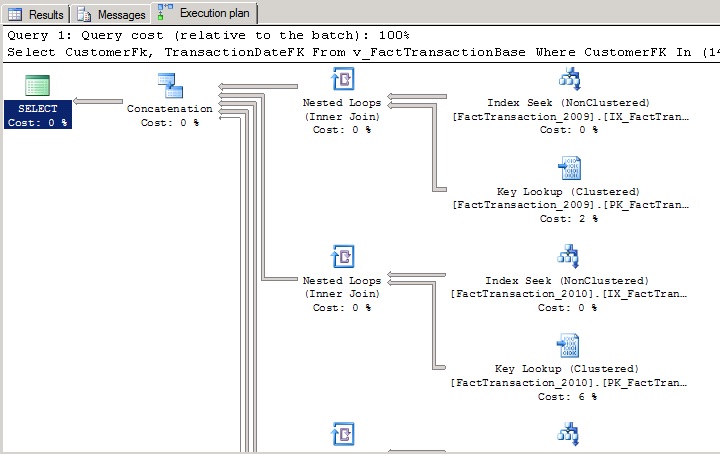
The below execution plan is displaying the query against the view. Notice the concatenation of the several individual queries on the Transaction tables. Please note that the image below is only displaying a part of the execution plan (select from 2009 and 2010) because the whole plan didn't fit on screen.

 3) Scenario 3

 In this scenario, I'm comparing an Update statement.

SET STATISTICS IO ON
UPDATE FactTransaction_ALL
    SET CustomerFK = CustomerFK
    WHERE CustomerFk IN ( 3175951, 1354109, 4788840, 5426872, 598353, 1300747,
                          3838935, 1300129, 1299711, 431263 )
        AND TransactionDateFK = 20130102
UPDATE FactTransaction
    SET CustomerFK = CustomerFK
    WHERE CustomerFk IN ( 3175951, 1354109, 4788840, 5426872, 598353, 1300747,
                          3838935, 1300129, 1299711, 431263 )
        AND TransactionDateFK = 20130102
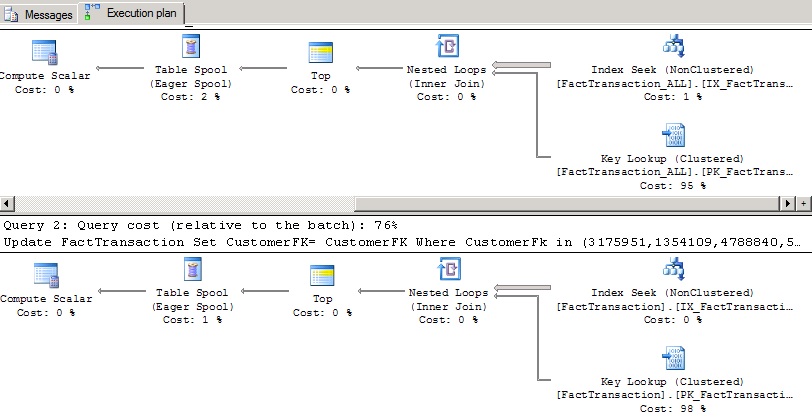
SET STATISTICS IO OFF

 As detailed below, it's more expensive to update the same number of rows on the big table than the small table.

Table 'FactTransaction_ALL'. Scan count 10, logical reads 126428, physical reads 0, read-ahead reads 0, lob logical reads 0, lob physical reads 0, lob read-ahead reads 0.

Table 'Worktable'. Scan count 1, logical reads 153, physical reads 0, read-ahead reads 0, lob logical reads 0, lob physical reads 0, lob read-ahead reads 0.

(75 row(s) affected)

(1 row(s) affected)

Table 'FactTransaction'. Scan count 10, logical reads 23079, physical reads 0, read-ahead reads 0, lob logical reads 0, lob physical reads 0, lob read-ahead reads 0.

Table 'Worktable'. Scan count 1, logical reads 153, physical reads 0, read-ahead reads 0, lob logical reads 0, lob physical reads 0, lob read-ahead reads 0.

(75 row(s) affected)

(1 row(s) affected)

Looking at the first update, 126,428 logical reads were needed while 23,079 reads were needed for the 2nd Update.

Advantages of Partitioned Views

Here are a few advantages from my point of view:

1. More control on DBCC commands and therefore faster execution.

On large databases,  a DBCC CHECKDB can take long hours, if not days, to complete and therefore the job is normally split across multiple days, invoking the CHECKTABLE command instead of the CHECKDB to perform a more tailored/specific table run. Thanks to multiple tables, (some of which may be read-only since they will not get updated), CHECKTABLE will only need to be executed against the current active table (which will be much smaller than the whole data set) with the benefit that it would finish before. 

2. Better space utilization.

Old and less queried data can be placed on less expensive RAID controllers. Current data will always make sense to store on fast RAID 10 while placing the old data on a slower and cheaper RAID 5 drive setup.

I would recommend Glenn Berry's SQL Server Hardware Book for a good explanation on SQL Server hardware and RAID Controllers.

3. More accurate Statistics

I will not be going into the internals of SQL Server statistics here, however since there will be less data in each table and the statistics histrogram is set to 200 steps, the histogram distribution would better reflect the data distribution. This will help the optimizer to select a better execution plan.

I would recommend Benjamin Nevarez Inside the SQL Server Query Optimizer Book for a good explanation on how the optimizer works.

4. Faster Statistics recomputations

As can be seen below, statistics computing is a huge advantage because the time will be drastically reduced. It's useless re-computing statistics for data which never changed and in this case, we'll be specifying which tables we'll be working on. For example, if we're in 2013, we'll re-compute statitics for the 2013 table only. On the other hand, if the data resides all in the same table, there is no way to recompute statistics for only a subset of the data, i.e. recompute data for a specific period only, or for a specific SQL Server table partition.

 5. More frequent statistics updates.

Statistics are updated when 20% of the data + 500 rows are changed. Therefore statistics on table FactTransaction_ALL will get updated when 20% of 141 millions rows i.e. 28 million rows get updated. On the other hand, the FactTransaction table that contains data just for 2013 will get updated when 20% of 27 million rows i.e. 5.4 millions rows get updated. 

As can be clearly observed, the 2nd table statistics will get updated more regulary, thus more updated statistics.

6. Smaller Tables and therefore MUCH more managable.

Let's say that I need to either add a new column to my huge table or change a column datatype, things that do happen even on a finished and stable system. Well from my experience, this will be a nightmare especially on the production server. The SQL statement below is an example;

Alter Table FactTransaction Alter Column <NewColumnFK> BigInt Not Null; 

On the production server, the above statement executed in 6 hours, in addition to the large amount of log space that was required to execute this change. Basically, I needed to add a new column to the fact table, populate it with data, then change it to 'Not Null' (statement above) and finally create and enforce a foreign key constraint. If the table has less data, such metadata changes will execute in a much more reasonable time.

Disadvantages of Partitioned Views

There are a few disadvantages to this approach as well

1. Application aware.

In my opinion, this is one of the major drawbacks to partitioned views. If the applications (being SSRS reports, OLAP Cube, Dashboards etc) were written with this in mind, i.e. all queries are executed against views, instead of the base tables, then this change would be minimal and can be implemented at a later day. Redirecting all table operations to a view can be a huge job.

2. Partitioning Columns.

This can also be a huge change to perform on an already live database, since it will involve changing the table's primary key & any Foreign key columns. One of the Partitioning Column rules clearly states that 'The partitioning column must be a part of the primary key of the table.'  

In the examples above, I skipped this part due to the changes which will be needed! I can still use the querying benefits of partitioned views however I cannot issue any DML statements directly against the view. Instead I have to update directly the corresponding base table. No big deal in my case.

 References

Using Partitioned Views in SQL Server 2008.

Creating Distributed Partitioned Views.

Views in SQL Server 2012

SET STATISTICS IO

DBCC CHECKDB